Validation: src/calliope/solve.py
What this page checks
This page checks the equilibrium solve in src/calliope/solve.py.
The solve finds the partial pressures of the gas and the dissolved masses for a given inventory of H, C, N, S and O.
Validation here means that we run the code on a case where another source gives the right answer.
The test then checks that the code gives that answer within a stated tolerance.
On this page the right answer comes from a second CALLIOPE solve that must agree with the first, from a closed-form result for the noble gases, and from a second code, atmodeller, for the gas-only grid.
If the solve is wrong, every outgassing step of a PROTEUS run gets the wrong atmosphere.
Each case below says why the check exists, what it tests, how we know the right answer and why it matters.
A box "Test details" at the end of each case gives the reference, the tolerance, the test id and the command.
The cases of the solve with a metal reservoir are on the metal reservoir page.
The 2 ways to call the solve.
The O budget is the mass of O in the gas and the melt together, O_kg_total [kg].
The buffered solve, equilibrium_atmosphere(target, ddict), takes the oxygen fugacity as input: you give the shift \(\Delta\mathrm{IW}\) from the iron-wüstite (IW) buffer in log10 units in ddict['fO2_shift_IW']. It returns the partial pressures, the mass of each species and the O budget that goes with them.
The authoritative-O solve, equilibrium_atmosphere_authoritative_O(target, ddict), takes the O budget as input in target['O'] and finds the \(\Delta\mathrm{IW}\) that matches it.
It treats the oxygen fugacity as a fifth unknown and solves the 5 by 5 mass balance of the 4 primary partial pressures (H\(_2\)O, CO\(_2\), N\(_2\), S\(_2\)) and the oxygen fugacity.
The metal reservoir page uses the same 2 names, and the authoritative oxygen page explains the second solve.
Terms used on this page.
- dex: a difference in log10 units; 0.05 dex is a factor of \(10^{0.05} \approx 1.12\).
- Regression snapshot: a set of stored values, results the code gave before. A test that compares with them fails when a result changes, but it does not show that the result is right.
- Cross-code check: a test that compares CALLIOPE with a second, independent code.
- atmodeller: an outgassing code that PROTEUS can use in place of CALLIOPE.
Round trip between the 2 solves
Why this check exists. The 2 solves share one chemistry. The buffered solve computes the O budget from the gas and melt that it finds; the authoritative-O solve must reach a given O budget. An error in how either solve counts O, or in the search for \(\Delta\mathrm{IW}\), makes the 2 solves disagree on the same planet.
What it tests. An Earth-like planet: \(T\) = 1800 K, a fully molten mantle of 4.03e24 kg, budgets of 1.5e20 kg H, 1.5e19 kg C, 8.0e18 kg N and 8.0e20 kg S, every volatile species included, and the default IW buffer. The buffered solve with \(\Delta\mathrm{IW}\) = 2 gives an O budget of 1.2254e21 kg; the test requires it between 1e18 and 1e22 kg. The authoritative-O solve with that O budget must then find \(\Delta\mathrm{IW}\) = 2 to 0.05 dex. With the random seeds of the test it finds 2.0000. With 5 other random starts of the buffered solve, the found \(\Delta\mathrm{IW}\) moved by at most 1.4e-4.
How we know the right answer. The authoritative-O solve starts from the O budget of the buffered solve, so the exact answer is the \(\Delta\mathrm{IW}\) of the buffered solve (a check of one code against itself).
Why it matters. PROTEUS uses the buffered solve with planet.fO2_source = "user_constant" and the authoritative-O solve with "from_O_budget". The 2 settings must describe the same planet the same way.
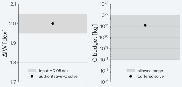
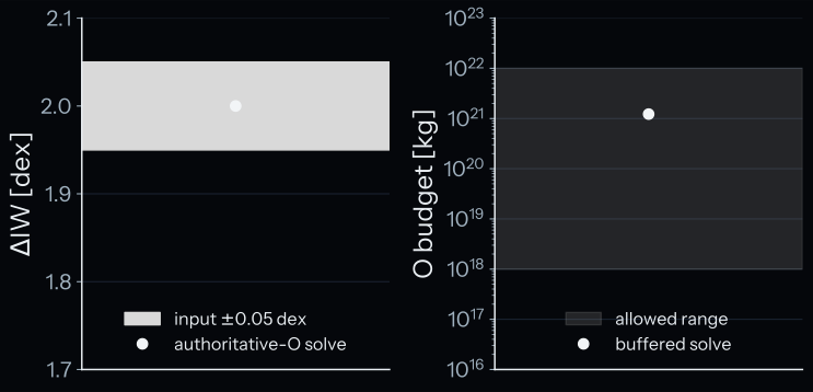
How to read the plot. The left panel shows the \(\Delta\mathrm{IW}\) that the authoritative-O solve finds, with the band of \(\pm 0.05\) dex around the input 2. The right panel shows the O budget of the buffered solve on a log axis, with the allowed range of 1e18 to 1e22 kg. A pass means that both marks lie inside their grey areas.
Test details
- Reference: cross-check of the 2 CALLIOPE solves:
equilibrium_atmosphereagainstequilibrium_atmosphere_authoritative_O. - Tolerance: 0.05 dex on the recovered \(\Delta\mathrm{IW}\); O budget between 1e18 and 1e22 kg.
- Test id:
tests/test_solve.py::test_round_trip_self_consistency_at_earth_fiducial - Command:
pytest tests/test_solve.py -k round_trip_self_consistency
Noble gases between melt and atmosphere
Why this check exists. The solve puts each noble gas into the melt by its Henry constant and into the atmosphere by its partial pressure. A wrong formula for the mass of the gas column, a wrong prefactor of the dissolved mass, or the constant of one gas used for another gives the wrong split.
What it tests. An Earth-scale magma ocean (\(T\) = 1800 K, fully molten mantle of 4.0e24 kg, gravity 9.81 m s\(^{-2}\), radius 6.37e6 m) with the species H\(_2\)O, CO\(_2\), N\(_2\) and S\(_2\) and the noble gases. For He, Ar and Xe the ratio of the dissolved mass to the atmospheric mass after the solve must equal the closed-form ratio to a relative 1e-6. For He the ratio must lie between 0 and 10.
How we know the right answer. For a noble gas the dissolved mass is \(10^{-6}\,M_\mathrm{mantle}\,\Phi\,k\,p\) and the atmospheric mass is \(10^5\,(A/g)\,(M/\mu)\,p\). Here \(p\) [bar] is its partial pressure, \(k\) [ppmw bar\(^{-1}\)] its Henry constant of Jambon et al. (1986), \(\Phi\) the melt fraction, \(A = 4\pi R^2\) the surface area, \(g\) the gravity, \(M\) its molar mass and \(\mu\) the mean molar mass of the gas. The ratio of the 2 does not depend on \(p\) (an analytical limit). The test takes \(\mu\) from the result of the solve, so it checks how the solve assembles the 2 masses, not the value of \(\mu\). The value of \(k\) itself is checked on the solubility page.
Why it matters. This split decides how much of each noble gas the atmosphere holds, and so how much escape can remove.
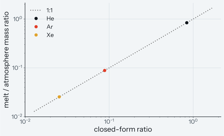
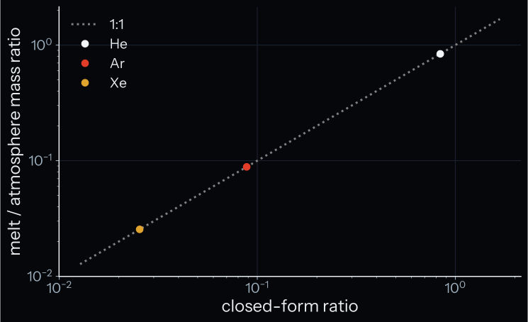
How to read the plot. Both axes are logarithmic. Each mark is one gas: the closed-form ratio on the x-axis and the ratio after the solve on the y-axis. A pass means that every mark lies on the dotted 1:1 line, to a relative 1e-6.
Test details
- Reference: analytical limit, the ratio of the Henry coefficient to the coefficient of the hydrostatic column.
- Tolerance: relative 1e-6 for He, Ar and Xe; \(0 < M_\mathrm{liquid}/M_\mathrm{atm} < 10\) for He.
- Test id:
tests/test_noble_gases.py::test_partition_ratio_matches_henry_versus_hydrostatic_column - Command:
pytest tests/test_noble_gases.py -k partition_ratio_matches_henry
Gas-only grid against atmodeller
Why this check exists. If the 2 codes give different gases for the same planet, a run changes when you change the code. This case finds a change in either code that moves the 2 apart.
What it tests. 72 cases with gas only, of a planet of 5.972e24 kg with a radius of 6335 km, a core mass fraction of 0.325 and no melt.
The reference inventory is 1.55e20 kg of H, the mass of the hydrogen in one Earth ocean of water (ocean_moles in constants.py), the same mass of C and of S, and half that mass of N. The cases are 3 inventories (0.1, 1 and 10 times the reference) at 4 temperatures (1500, 2000, 2500 and 3000 K). For 60 cases both codes get the same \(f\mathrm{O_2}\), at \(\Delta\mathrm{IW}\) = -4, -2, 0, +2 and +4 of the Fischer buffer. The other 12 cases give both codes an O budget. For each case the test requires:
- that atmodeller converges in every case;
- in the 60 buffered cases, that the gas of CALLIOPE holds each element budget to 1e-5 of the largest budget plus 1e10 kg plus 10 kg;
- in the 12 O-budget cases, that it holds each element budget to 1e-5 of that budget or 10 kg, whichever is larger, and that the O budget of both codes holds to a relative 1e-9;
- the offset \(\log_{10}(p_\mathrm{CALLIOPE}/p_\mathrm{atmodeller})\) of the surface pressure and of 10 species (11 in the O-budget cases), no more than 0.005 dex from its stored offset;
- in the O-budget cases a tighter bound of 0.001 dex for the surface pressure and for H\(_2\)O, CO\(_2\), N\(_2\), SO\(_2\) and S\(_2\);
- the offset of the SO\(_2\) reaction quotient, no more than 0.002 dex from its stored offset.
How we know the right answer. The 2 codes use different fits of the thermodynamic data, so the expected offsets are not zero: they are stored values, a regression snapshot. The largest stored offset is that of CH\(_4\), 0.109 dex. Before the solves, the test checks that the NASA Glenn values1 of the chemistry page equal atmodeller's own polynomials to 1e-6 in \(\log_{10} K\).
Why it matters. The cross-code comparison of CALLIOPE and atmodeller depends on the size of these known offsets, and this case fails if an offset moves by more than its bound.
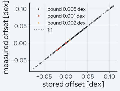
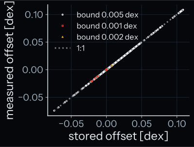
How to read the plot. Each mark is one checked quantity of one case: its stored offset on the x-axis and the offset measured in the test on the y-axis. The shape gives the bound of the check. Circles have 0.005 dex. Squares have 0.001 dex: the surface pressure, H\(_2\)O, CO\(_2\), N\(_2\), SO\(_2\) and S\(_2\) of the O-budget cases. Triangles have 0.002 dex: the SO\(_2\) quotient. A pass means that every mark lies on the dotted 1:1 line within its bound. The bounds are too small to see at this scale, and many circles overlap along the line. The element and O closure checks and the report-file check are not drawn.
Known limit. The offsets are a regression snapshot: the case fails if an offset moves, but it does not say which code is right. The grid has no melt, so it does not compare the solubility laws of the 2 codes. It runs only in the nightly cross-code job, because it needs atmodeller. The comparison at the Earth case in scripts/cross_backend/ is not part of the test suite.
Test details
- Reference: atmodeller (cross-code check).
- Tolerance: element budgets of CALLIOPE to 1e-5 of the largest budget plus 1e10 kg plus 10 kg (buffered) or to 1e-5 of each budget, at least 10 kg (O budget), O budget of both codes to a relative 1e-9; each offset no more than 0.005 dex from its stored value (0.001 dex for the surface pressure, H\(_2\)O, CO\(_2\), N\(_2\), SO\(_2\) and S\(_2\) with an O budget); SO\(_2\) quotient to 0.002 dex.
- Test id:
tests/test_cross_code_consistency.py::test_calliope_vs_atmodeller_72_case_gas_only_grid - Command:
pytest tests/test_cross_code_consistency.py -k 72_case(integration tier; skips without atmodeller)
Other tests of the solve
solve.py is a large file, so its tests are split by topic:
tests/test_authoritative_O.pyand the filestest_authoritative_O_*.py: the contract of the authoritative-O solve, its monotonicity and its input checks.tests/test_equilibrium_paths.py: the buffered solve on compositions with many species.tests/test_partial_species.py: solves with some elements left out.tests/test_stoichiometry.py: the stoichiometric ratios of the reactions.tests/test_targets.py: the element budgets.tests/test_noble_gases.py: the noble gases (He, Ne, Ar, Kr, Xe): their split, mass closure, their effect on the mean molar mass, and their budgets.tests/test_invariants.py: closure of every element and species.tests/test_invariants_hypothesis.py: property-based tests at the slow tier.
Related code and pages
src/calliope/solve.py: the 2 solves.- Authoritative oxygen: the explanation page of the authoritative-O solve.
- Cross-code comparison: CALLIOPE with the Fischer buffer against atmodeller with the Hirschmann buffer at the Earth case, with a residual of 0.16 dex in \(\Delta\mathrm{IW}\).
References
-
B. J. McBride, M. J. Zehe, S. Gordon, NASA Glenn Coefficients for Calculating Thermodynamic Properties of Individual Species, NASA/TP-2002-211556, NASA Glenn Research Center, 2002. ↩