Coupled-loop driver

The most common real-world use of CALLIOPE is inside a time-stepping outer loop that advances a magma ocean through cooling, escape, or any other process that re-equilibrates the atmosphere at each step. This tutorial shows the warm-start pattern that makes such loops efficient.

By the end of it you will:

• have written a minimal driver that calls CALLIOPE at each time step;
• know which fields to thread between iterations as p_guess;
• have measured the warm-start speed-up directly: cold-start solve vs warm-start solve;
• have run two phases back-to-back on the same warm-start chain: a cooling sequence from \(T_\mathrm{magma} = 3000\) K to \(1500\) K at \(\Phi = 1\), then a crystallisation step at fixed \(T = 1500\) K where the melt fraction drops from \(\Phi = 1\) to \(\Phi = 0.5\);
• have produced the two-panel partial-pressure plot on the front of this page.

You should already have completed the First run tutorial. Familiarity with Two-mode round-trip is helpful but not required.

What "warm start" means in CALLIOPE

CALLIOPE's equilibrium_atmosphere solves a 4-by-4 nonlinear mass-balance system in the partial pressures \((p_\mathrm{H_2O}, p_\mathrm{CO_2}, p_\mathrm{N_2}, p_\mathrm{S_2})\). Without an initial guess, it draws Monte-Carlo log-uniform restarts (up to nguess, default 7500) until fsolve converges to a basin that satisfies mass balance. With a p_guess dictionary close to the solution, fsolve typically converges on the first attempt and the call completes in a few milliseconds rather than tens to hundreds.

In a time-stepping loop where the chemistry changes slowly (i.e. each step is a small perturbation of the previous), the previous step's converged partial pressures are an excellent guess for the next. This is the warm-start pattern.

Step 1: write a cooling-sequence driver

import time
import warnings

import numpy as np

from calliope.constants import volatile_species
from calliope.solve import equilibrium_atmosphere

planet = {'M_mantle': 4.03e24, 'gravity': 9.81, 'radius': 6.371e6}
earth_hcns = {'H': 5.6e20, 'C': 3.1e21, 'N': 3.7e19, 'S': 1.0e21}

T_sequence = np.linspace(3000.0, 1500.0, 25)
diw_fixed  = 0.5            # hold redox fixed: the focus is cooling

species_to_track = ['H2O', 'CO2', 'H2', 'CO', 'CH4',
                    'N2', 'NH3', 'S2', 'SO2', 'H2S']
history = {sp: np.full(T_sequence.size, np.nan) for sp in species_to_track}
wall    = np.zeros(T_sequence.size)

p_guess = None             # cold-start the first call

Step 2: the loop, with warm-start threading

for i, T in enumerate(T_sequence):
    ddict = {**planet, 'T_magma': float(T), 'Phi_global': 1.0,
             'fO2_shift_IW': diw_fixed}
    for sp in volatile_species:
        ddict[f'{sp}_included']    = 1
        ddict[f'{sp}_initial_bar'] = 0.0

    t0 = time.time()
    with warnings.catch_warnings():
        warnings.simplefilter('ignore')
        res = equilibrium_atmosphere(
            earth_hcns, ddict, p_guess=p_guess, print_result=False,
        )
    wall[i] = time.time() - t0

    for sp in species_to_track:
        history[sp][i] = float(res[f'{sp}_bar'])

    # Thread the four primary partial pressures forward as the next
    # iteration's guess. Other species are derived from these four via
    # the equilibrium reactions, so re-seeding them is not necessary.
    p_guess = {s: float(res[f'{s}_bar']) for s in ('H2O', 'CO2', 'N2', 'S2')}

print(f'cold-start step: {wall[0]*1e3:6.1f} ms')
print(f'warm-step median: {np.median(wall[1:])*1e3:6.1f} ms')

You should see the warm steps run several times faster than the cold start. The exact ratio depends on how lucky the cold-start Monte-Carlo draw is on the first call: when the draw is lucky the cold call already converges quickly and the warm steps are only a few-fold faster (~3x in the cached run on this page); when the cold draw needs many restarts the warm-step speed-up can be an order of magnitude or more.

Step 3: crystallisation at fixed temperature

A real magma ocean does more than cool monotonically: at some point the solidus catches the geotherm and the magma begins to crystallise, dropping the melt fraction \(\Phi\). CALLIOPE's \(\Phi\) parameter controls how much of the silicate reservoir participates in melt-vapour equilibrium, so reducing \(\Phi\) at fixed \(T\) progressively shrinks the magma reservoir and rebalances the H, C, N, S partitioning between melt and atmosphere.

Continue the same warm-start chain from the end of the cooling sequence and walk \(\Phi\) from \(1.0\) down to \(0.5\) at fixed \(T = 1500\) K:

phi_grid = np.linspace(1.0, 0.5, 11)
cryst_history = {sp: np.full(phi_grid.size, np.nan) for sp in species_to_track}

# p_guess and ddict carry over from the end of Step 2.
for j, phi in enumerate(phi_grid):
    ddict['T_magma']    = 1500.0
    ddict['Phi_global'] = float(phi)
    with warnings.catch_warnings():
        warnings.simplefilter('ignore')
        res = equilibrium_atmosphere(
            earth_hcns, ddict, p_guess=p_guess, print_result=False,
        )
    for sp in species_to_track:
        cryst_history[sp][j] = float(res[f'{sp}_bar'])
    p_guess = {s: float(res[f'{s}_bar']) for s in ('H2O', 'CO2', 'N2', 'S2')}

As \(\Phi\) drops, the partial pressures of the dissolved-friendly species (H\(_2\)O above all, then SO\(_2\), NH\(_3\), H\(_2\)S) rise: shrinking the melt reservoir squeezes the previously-dissolved volatiles into the atmosphere. The barely-soluble species (CO, CO\(_2\), N\(_2\)) move comparatively little because they were already outgassed at \(\Phi = 1\).

Step 4: plot both phases

import matplotlib.pyplot as plt

from calliope.constants import dict_colors

fig, (ax_cool, ax_cryst) = plt.subplots(
    1, 2, figsize=(11.4, 5.0), sharey=True,
    gridspec_kw={'width_ratios': [1.6, 1.0], 'wspace': 0.08},
)

for sp in species_to_track:
    ax_cool.plot(T_sequence, history[sp],
                 color=dict_colors[sp], marker='o', markersize=3.5,
                 linewidth=1.8)
    ax_cryst.plot(phi_grid, cryst_history[sp],
                  color=dict_colors[sp], marker='s', markersize=3.5,
                  linewidth=1.8, label=sp)
ax_cool.set_yscale('log')
ax_cool.set_xlabel(r'$T_\mathrm{magma}$ [K] (cooling $\rightarrow$)')
ax_cool.set_ylabel('Surface partial pressure (bar)')
ax_cool.set_ylim(1e-6, 1e4)
ax_cool.invert_xaxis()
ax_cool.grid(which='both', alpha=0.3)
ax_cool.set_title(r'(a) cooling at $\Phi = 1$')
ax_cryst.set_xlabel(r'$\Phi_\mathrm{global}$ (crystallisation $\rightarrow$)')
ax_cryst.invert_xaxis()
ax_cryst.grid(which='both', alpha=0.3)
ax_cryst.set_title(r'(b) crystallisation at $T = 1500$ K')
ax_cryst.legend(loc='center left', bbox_to_anchor=(1.02, 0.5), frameon=False)
fig.savefig('coupled_loop.pdf')

The goal of this tutorial

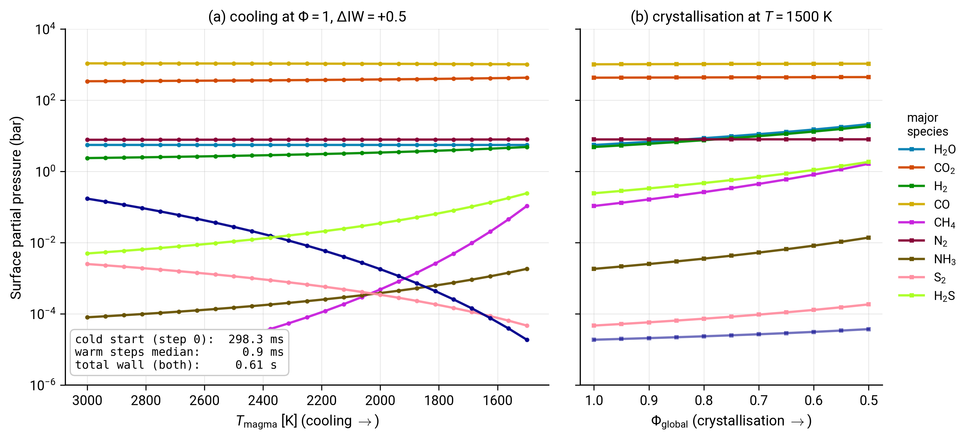
Surface partial pressures across a two-phase driver. (a) A 25-step cooling sequence from \(3000\) K down to \(1500\) K at fixed \(\Phi = 1\) and \(\Delta\mathrm{IW} = +0.5\). (b) An 11-step crystallisation step at fixed \(T = 1500\) K with the magma melt fraction shrinking from \(\Phi = 1\) to \(\Phi = 0.5\). The legend lists the ten tracked species in their PROTEUS-standard colours; the annotation in panel (a) shows the cold-start time (first call), the warm-step median (every subsequent call), and the total wall time for the full \(25 + 11\) steps.

In panel (a) the atmosphere stays carbon-dominated across the whole cooling range; CO is the dominant species throughout (CO/CO\(_2\) ratio falls modestly as \(T\) drops). The fastest-moving species are H\(_2\)S (rises) and S\(_2\) (falls): sulfur speciation is the most sensitive marker of cooling at this redox.

Panel (b) shows the magma-volume effect cleanly. As \(\Phi\) drops the dissolved-friendly species (H\(_2\)O above all, plus the trace S species) rise sharply because the shrinking melt reservoir pushes them into the atmosphere; the barely-soluble species (CO, CO\(_2\), N\(_2\)) move comparatively little. The total surface pressure rises by tens of percent across the \(\Phi = 1 \to 0.5\) step, almost entirely driven by the H\(_2\)O / H\(_2\)S / SO\(_2\) surge.

The wall-time annotation is the most pedagogically important number on the plot. The total wall time is dominated by the cold-start step; warm steps are typically order milliseconds each across both phases, even though phase 2 changes a different state variable than phase 1. This is what makes long PROTEUS runs (\(10^4\) or more outer-loop iterations) feasible: each CALLIOPE call costs essentially nothing once the basin is found.

Where to go next

• For the conceptual story behind the equilibrium chemistry CALLIOPE is solving, read Equilibrium chemistry.
• For the PROTEUS-side wrapper that implements this pattern in production, read Coupling to PROTEUS.
• For how CALLIOPE behaves when the inputs vary more aggressively across the (T, \(\Delta\mathrm{IW}\)) plane, see the previous tutorial Speciation phase diagram.

Reproducing the figure

Generated by scripts/tutorials/fig_coupled_loop.py. Re-run with python -m scripts.tutorials.fig_coupled_loop from the repository root.