Reproducing the Earth fiducial

The Backend comparison explanation page anchors all of its figures on one shared Earth scenario: Krijt et al. 2023² BSE H/C/N/S, \(T_\mathrm{magma} = 2000\) K, \(\Phi = 1\), and a volatile O reference of \(1.26 \times 10^{22}\) kg derived to put CALLIOPE on the Sossi et al. 2020³ \(\Delta\mathrm{IW} = +3.5\) Earth upper-mantle anchor with the current default Fischer 2011 buffer. This tutorial walks you through reproducing those numbers from scratch so you can verify the docs are still consistent with the current solver, and so you have the workflow on hand when you want to anchor your own runs to a literature value.

By the end of it you will:

• have reproduced the \(O = 1.26 \times 10^{22}\) kg volatile-O reference from the Krijt H/C/N/S budget;
• have verified that the authoritative-O entry point recovers \(\Delta\mathrm{IW} = +3.5\) from that O reference to within solver tolerance;
• understand why the buffered call at high \(\Delta\mathrm{IW}\) + carbon-rich BSE needs a tight p_guess (it has a spurious secondary basin without it).

You should already have completed Two-mode round-trip, which introduces both entry points.

Step 1: pin the Krijt+2023 H/C/N/S budget

import warnings

from calliope.constants import volatile_species
from calliope.solve import (
    equilibrium_atmosphere,
    equilibrium_atmosphere_authoritative_O,
)

planet  = {'M_mantle': 4.03e24, 'gravity': 9.81, 'radius': 6.371e6}
T_magma = 2000.0
diw_anchor = 3.5   # Sossi et al. 2020 Earth upper-mantle estimate

# Krijt et al. 2023 PPVII Tables 1 and 2 BSE row (kg).
earth_hcns = {'H': 5.6e20, 'C': 3.1e21, 'N': 3.7e19, 'S': 1.0e21}

Step 2: derive the volatile-O reference via buffered mode

This is the step that needs the tight p_guess.

Without one, the buffered solver at high \(\Delta\mathrm{IW}\) with a carbon-rich BSE inventory has two basins: the physical CO\(_2\)-dominated one at \(P_\mathrm{surf} \approx 1755\) bar with \(p_\mathrm{H_2O} \approx 5.6\) bar, and a spurious H\(_2\)O-free one at lower \(P_\mathrm{surf}\) with \(p_\mathrm{H_2O} = 0\). The Monte-Carlo restart lands in the spurious basin a few percent of the time, which is rare but too often for a reproducible tutorial.

A p_guess near the CO\(_2\)-dominated basin pins the right answer reliably:

ddict = {**planet, 'T_magma': T_magma, 'Phi_global': 1.0,
         'fO2_shift_IW': diw_anchor}
for sp in volatile_species:
    ddict[f'{sp}_included']    = 1
    ddict[f'{sp}_initial_bar'] = 0.0

# Pin the canonical CO2-dominated basin. Numbers are approximate; the
# solver tightens them to the converged values during fsolve.
canonical_guess = {'H2O': 5.0, 'CO2': 1500.0, 'N2': 3.0, 'S2': 1e-3}

with warnings.catch_warnings():
    warnings.simplefilter('ignore')
    buf = equilibrium_atmosphere(
        earth_hcns, ddict, p_guess=canonical_guess, print_result=False,
    )

print(f'derived O_kg_total = {buf["O_kg_total"]:.3e} kg')
print(f'P_surf            = {buf["P_surf"]:.0f} bar')
print(f'H2O               = {buf["H2O_bar"]:.2f} bar')
print(f'CO2               = {buf["CO2_bar"]:.0f} bar')

Expected output:

derived O_kg_total = 1.260e+22 kg
P_surf            = 1755 bar
H2O               = 5.59 bar
CO2               = 1557 bar

This is the canonical Earth volatile-O reference under the current Fischer 2011 buffer default and matches the value used on the backend-comparison page.

Step 3: round-trip through authoritative-O

Feed the derived O budget into the authoritative-O entry point and verify that it recovers the input \(\Delta\mathrm{IW}\) within solver tolerance:

target = dict(earth_hcns); target['O'] = buf['O_kg_total']
p_guess = {s: float(buf[f'{s}_bar']) for s in ('H2O', 'CO2', 'N2', 'S2')}

with warnings.catch_warnings():
    warnings.simplefilter('ignore')
    auth = equilibrium_atmosphere_authoritative_O(
        target, ddict, p_guess=p_guess, fO2_hint=diw_anchor,
        print_result=False,
    )

residual = auth['fO2_shift_derived'] - diw_anchor
print(f'recovered Delta-IW = {auth["fO2_shift_derived"]:+.4f}')
print(f'residual           = {residual:+.2e} dex')

Expected output: residual \(\lesssim 10^{-9}\) dex, i.e. essentially zero (the exact value depends on solver tolerance and starting point). The full provenance chain (Krijt H/C/N/S \(\to\) buffered mode \(\to\) derived O \(\to\) authoritative-O \(\to\) \(\Delta\mathrm{IW}\)) closes at the Sossi 2020 anchor.

The goal of this tutorial

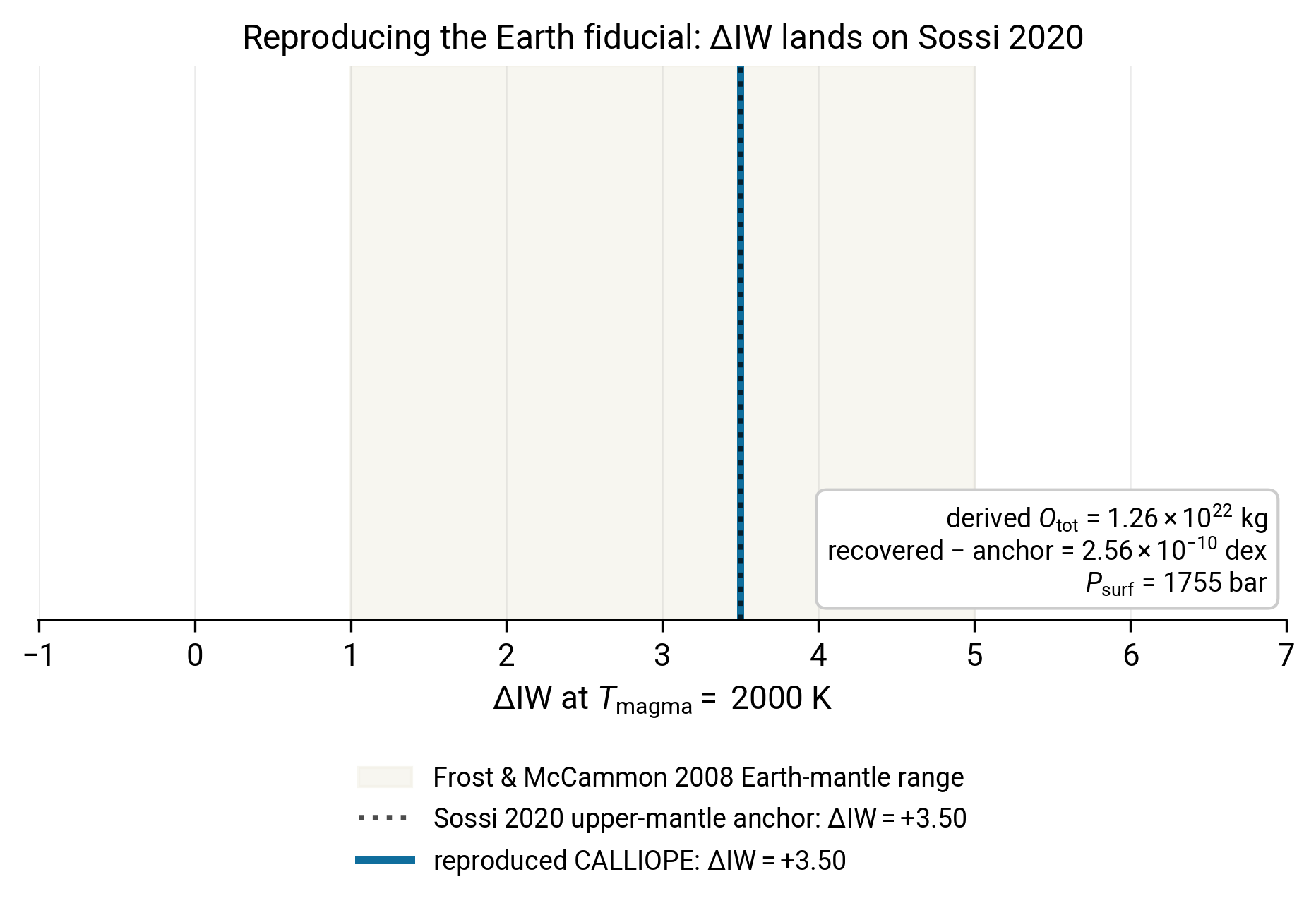
Earth fiducial reproduced from scratch. The cream band represents the Frost & McCammon 2008¹ empirical Earth-mantle range, \(\Delta\mathrm{IW} \in [+1, +5]\) (a conversion of their stated FMQ \(\pm 2\) dex upper-mantle window onto the IW reference). The dotted vertical is the Sossi et al. 2020³ upper-mantle anchor, \(\Delta\mathrm{IW} = +3.50\). The solid line is the CALLIOPE recovered value after the buffered \(\to\) authoritative-O round-trip. The summary box reports the derived O budget, the absolute closure residual (a few parts in \(10^9\)), and the converged surface pressure. The reproduced CALLIOPE line sits exactly on the Sossi anchor, as it should: the entire workflow is constructed to land on this value.

If your reproduced figure does not show the CALLIOPE line on the Sossi anchor, the most likely cause is that you skipped the canonical_guess in Step 2 and the buffered solver landed in the spurious H\(_2\)O-free basin. Add the p_guess and re-run.

Where to go next

• For the full atmosphere-side details (every partial pressure at this fiducial), open the First-run reference figure and substitute these inputs.
• For how this fiducial sits inside the cross-backend story (CALLIOPE vs atmodeller at the same inputs), read the Backend comparison explanation page.
• For the planetary case study that contrasts Earth-BSE with a very different inventory, read the next tutorial: Mars-like atmosphere.

Reproducing the figure

Generated by scripts/tutorials/fig_earth_fiducial.py. Re-run with python -m scripts.tutorials.fig_earth_fiducial from the repository root.