Mars-like atmosphere

CALLIOPE is not Earth-specific. Anything in the planet parameter dictionary (M_mantle, gravity, radius) is a knob the user can change, and the solubility laws are calibrated against terrestrial-basalt melts that extrapolate reasonably to other rocky bodies. This tutorial swaps in Mars-like planetary parameters and a mass-scaled inventory, runs the same chemistry, and reads off how the atmosphere differs.

By the end of it you will:

• have run CALLIOPE on a non-Earth planet;
• have a side-by-side comparison of Earth-BSE and Mars-scaled atmospheres at the same redox and temperature;
• know which atmospheric properties are inventory-driven (per-species partial pressures) and which are structure-driven (surface pressure, atmospheric mass).

You should already have completed First run. The other tutorials are not strictly required but make the figure easier to interpret.

Step 1: define both planets

import warnings

import numpy as np

from calliope.constants import volatile_species
from calliope.solve import equilibrium_atmosphere

earth = {
    'name': 'Earth',
    'planet': {'M_mantle': 4.03e24, 'gravity': 9.81, 'radius': 6.371e6},
    'hcns':   {'H': 5.6e20, 'C': 3.1e21, 'N': 3.7e19, 'S': 1.0e21},
}

mass_ratio = 0.107  # Mars / Earth
mars = {
    'name': 'Mars-scaled',
    'planet': {'M_mantle': 5.03e23, 'gravity': 3.71, 'radius': 3.39e6},
    'hcns':   {k: v * mass_ratio for k, v in earth['hcns'].items()},
}

T_magma = 2500.0
diw     = 0.5
phi     = 1.0

Step 2: solve each planet's atmosphere

def solve_atmosphere(cfg):
    ddict = {**cfg['planet'], 'T_magma': T_magma, 'Phi_global': phi,
             'fO2_shift_IW': diw}
    for sp in volatile_species:
        ddict[f'{sp}_included']    = 1
        ddict[f'{sp}_initial_bar'] = 0.0
    with warnings.catch_warnings():
        warnings.simplefilter('ignore')
        return equilibrium_atmosphere(cfg['hcns'], ddict, print_result=False)

earth_out = solve_atmosphere(earth)
mars_out  = solve_atmosphere(mars)

print(f'Earth: P_surf = {earth_out["P_surf"]:6.1f} bar, M_atm = {earth_out["M_atm"]:.2e} kg')
print(f'Mars : P_surf = {mars_out["P_surf"]:6.1f} bar, M_atm = {mars_out["M_atm"]:.2e} kg')

You should see (current default Fischer 2011 buffer):

Earth: P_surf = 1449.4 bar, M_atm = 7.54e+21 kg
Mars : P_surf =  225.9 bar, M_atm = 8.79e+20 kg

Two things are worth noticing:

• The Mars atmosphere has about \(1/9\) the mass of Earth's, in line with the \(0.107\) inventory scaling. The chemistry is roughly mass-linear at this regime.
• The Mars surface pressure is only \(\sim 1/6\) of Earth's, not \(1/9\), because the smaller gravity (\(3.71\) m s\(^{-2}\) vs \(9.81\) m s\(^{-2}\)) trades against the smaller atmospheric mass: \(P_\mathrm{surf} = g M_\mathrm{atm} / (4\pi R^2)\), so the gravity ratio (\(0.38\)) partly compensates the mass ratio (\(0.11\)).

Step 3: plot the comparison

import matplotlib.pyplot as plt

from calliope.constants import dict_colors

species = ['H2O', 'CO2', 'H2', 'CO', 'CH4',
           'N2', 'NH3', 'S2', 'SO2', 'H2S']

# Sort by Earth pressure descending; Mars uses the same order so the
# comparison is bar-by-bar.
order = sorted(species, key=lambda sp: -earth_out[f'{sp}_bar'])
earth_p = np.array([earth_out[f'{sp}_bar'] for sp in order])
mars_p  = np.array([mars_out[f'{sp}_bar']  for sp in order])

fig, ax = plt.subplots(figsize=(8.0, 5.4))
y = np.arange(len(order)) * 1.8
h = 0.7
ax.barh(y - h / 2, earth_p, height=h,
        color=[dict_colors[sp] for sp in order],
        edgecolor='black', linewidth=0.5, label='Earth-BSE')
ax.barh(y + h / 2, mars_p, height=h,
        color=[dict_colors[sp] for sp in order], alpha=0.45,
        edgecolor='black', linewidth=0.5, hatch='///',
        label='Mars-scaled (0.107 x Earth inventory)')
ax.set_xscale('log')
ax.set_yticks(y)
ax.set_yticklabels(order)
ax.invert_yaxis()
ax.set_xlabel('Surface partial pressure (bar)')
ax.legend(loc='upper center', bbox_to_anchor=(0.5, -0.12), ncol=2, frameon=False)
fig.tight_layout()
fig.savefig('mars_vs_earth.pdf')

The goal of this tutorial

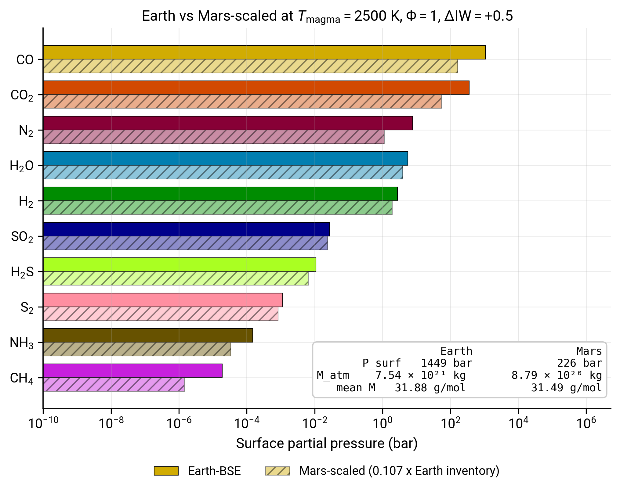
Surface partial pressures at \(T_\mathrm{magma} = 2500\) K, \(\Delta\mathrm{IW} = +0.5\), \(\Phi = 1\) on two bodies. Solid bars: Earth-BSE Krijt+2023 inventory on Earth planetary parameters. Hatched bars: same inventory scaled by Mars / Earth mass ratio (0.107) on Mars planetary parameters. Species ordered top-to-bottom by Earth partial pressure. Summary box top-right reports the three aggregate diagnostics for both bodies.

The figure makes one pedagogical point cleanly: at fixed redox and temperature, the per-species partial pressures on the Mars-scaled body track Earth's by roughly the same factor across the redox-relevant species (CO, CO\(_2\), N\(_2\), H\(_2\), H\(_2\)O). The dominant-species ordering is preserved: CO dominates on both bodies because the C / H mass ratio in the inventory is identical (we scaled uniformly). What changes is the absolute scale.

This is the right intuition to carry into more sophisticated planetary work. A genuinely different composition (different C / H, different volatile-element fractionation, a depleted N or S budget) will shift the dominant species and break the parallel-bar pattern. A genuinely different structure (Mars-mass body with Earth-mass mantle, or a Venus-mass body with Mars-fraction volatiles) will shift the surface pressure without shifting the speciation. The two effects separate cleanly because CALLIOPE's chemistry depends on element budgets, not on how those budgets were divided among Earth-mass and Mars-mass bodies.

A third change, and the one likely most relevant to real Mars work, would substantially break the parallel-bar pattern: the mantle redox state. The shergottite parent-melt estimate of Mars's upper-mantle \(f_{\mathrm{O}_2}\) from Wadhwa 2001³ spans roughly \(\Delta\mathrm{IW} \approx -1\) to \(\Delta\mathrm{IW} \approx +2\), more reducing than the Sossi 2020 \(\Delta\mathrm{IW} = +3.5\) Earth upper-mantle anchor used in this tutorial. The Speciation phase diagram tutorial shows that at \(\Delta\mathrm{IW} \lesssim +2\) the dominant species at this temperature flips from CO\(_2\) to CO, and that H\(_2\)O and CO\(_2\) drop sharply below the CO / H\(_2\) pair. A Mars run that takes the petrologically motivated \(\Delta\mathrm{IW} \sim +1\) instead of the \(\Delta\mathrm{IW} = +0.5\) used here would therefore see substantially less H\(_2\)O and a much more reducing atmosphere overall, separately from the planetary-structure scaling explored on this page.

Where to go next

• Swap in a literature Mars BSE inventory (Wänke & Dreibus 1988²) in the mars['hcns'] dict and re-run; compare the per-species shift to the uniform-scaling result.
• Reduce the redox to \(\Delta\mathrm{IW} = -3\) to look at a Mercury-like reducing endmember on the same Mars-mass body; the dominant species will switch.
• Read Equilibrium chemistry for the reactions that hold across all of these scenarios.

Reproducing the figure

Generated by scripts/tutorials/fig_mars_fiducial.py. Re-run with python -m scripts.tutorials.fig_mars_fiducial from the repository root.