First run

This tutorial walks an Earth-like volatile inventory through CALLIOPE and visualises the resulting atmosphere. By the end of it you will have called the equilibrium solver, read the output dictionary, and produced a partial-pressure plot you can adapt for your own work.

You should already have CALLIOPE installed (see Installation) and have read the Configuration page so the dictionary keys feel familiar.

Step 1: build the input

Open a fresh Python script (or notebook) and assemble the magma-ocean state:

import numpy as np
import matplotlib.pyplot as plt

from calliope.constants import volatile_species, dict_colors
from calliope.solve import equilibrium_atmosphere, get_target_from_params

ddict = {
    # planet
    'M_mantle': 4.03e24,    # kg, Earth mantle mass
    'gravity':  9.81,       # m s-2
    'radius':   6.371e6,    # m

    # magma ocean state
    'T_magma':      2500.0,  # K, hot magma ocean
    'Phi_global':   1.0,     # fully molten
    'fO2_shift_IW': 0.5,     # illustrative value: between IW (Bower+2022 use
                             # IW and IW+4 in their grid) and Sossi+2020's
                             # +3.5 estimate for Earth's surface mantle

    # bulk composition (Earth-ocean H, Earth-like C/H, primitive N and S)
    'hydrogen_earth_oceans': 1.0,
    'CH_ratio':              0.1,
    'nitrogen_ppmw':         2.0,
    'sulfur_ppmw':           200.0,
}

for sp in volatile_species:
    ddict[f'{sp}_included']    = 1     # include all 11 species
    ddict[f'{sp}_initial_bar'] = 0.0   # zero, not used in this mode (only
                                       # consulted by get_target_from_pressures)

Step 2: build the elemental targets and solve

target = get_target_from_params(ddict)
print('Target inventories [kg]:')
for el, kg in target.items():
    print(f'  {el}: {kg:.3e}')

result = equilibrium_atmosphere(target, ddict, print_result=False)

The first call may take a few seconds because CALLIOPE's Monte-Carlo initial-guess generator typically needs 10-50 restarts to find the right basin without a warm start. Subsequent calls with p_guess= from the previous result complete in tens of milliseconds.

Step 3: read the result

print(f"Surface pressure : {result['P_surf']:8.2f} bar")
print(f"Atmosphere mass  : {result['M_atm']:.3e} kg")
print(f"Mean mol. mass   : {result['atm_kg_per_mol'] * 1e3:6.3f} g/mol\n")

print('Surface partial pressures:')
for sp in sorted(volatile_species, key=lambda s: -result[f'{s}_bar']):
    p = result[f'{sp}_bar']
    x = result[f'{sp}_vmr']
    if p > 1e-6:
        print(f'  {sp:5s}: {p:9.3e} bar  (VMR {x:.3e})')

For the inputs above (1 ocean H, \(\Delta\mathrm{IW} = +0.5\), \(T = 2500\) K, \(\Phi = 1\)) you should see roughly a 10 bar atmosphere with CO dominant, then CO\(_2\), N\(_2\), and H\(_2\)O at the bar level, and H\(_2\) plus the S and N trace species below. The exact values depend on the solubility-law defaults; see Solubility laws for what each species uses.

Step 4: verify mass balance

The solver returns the final residual for each element (in kg). They should be small relative to the input target:

print('\nMass-balance residuals:')
for el in ['H', 'C', 'N', 'S']:
    res = result[f'{el}_res']
    rel = res / target[el]
    print(f'  {el}: {res:+.3e} kg  ({rel:+.2e} relative)')

A successful solve has \(|\text{res}_e| / \text{target}_e \lesssim 10^{-5}\) for every element. Larger residuals mean the tolerance was loose or the solver bottomed out on a local minimum; tighten rtol and re-run, or pass a p_guess from a known-good run.

Step 5: plot

O\(_2\) is set diagnostically by the \(f_{\mathrm{O}_2}\) buffer (it is not solved for), so the bar chart focuses on the ten reactive species:

species_to_plot = ['H2O', 'CO2', 'H2', 'CO', 'CH4', 'N2', 'NH3', 'S2', 'SO2', 'H2S']
pressures = np.array([result[f'{sp}_bar'] for sp in species_to_plot])
colors = [dict_colors[sp] for sp in species_to_plot]

fig, ax = plt.subplots(figsize=(7, 4))
ax.bar(species_to_plot, pressures, color=colors, edgecolor='black', linewidth=0.5)
ax.set_yscale('log')
ax.set_ylabel('Surface partial pressure (bar)')
ax.set_title(rf'$T = {ddict["T_magma"]:.0f}$ K, $\Phi = {ddict["Phi_global"]}$, $\Delta$IW $ = {ddict["fO2_shift_IW"]:+.1f}$')
ax.set_ylim(1e-6, 1e4)
ax.grid(axis='y', which='both', alpha=0.3)
fig.tight_layout()
fig.savefig('first_run.pdf')
plt.show()

dict_colors from calliope.constants is the colour scheme used across the PROTEUS ecosystem so figures stay visually consistent.

Compare your output against the reference

The figure below is the same Earth-like inputs run through equilibrium_atmosphere on a clean CALLIOPE install. Your numbers should reproduce these to within a few percent (the residual reflects Monte-Carlo restart variability, not a calibration issue).

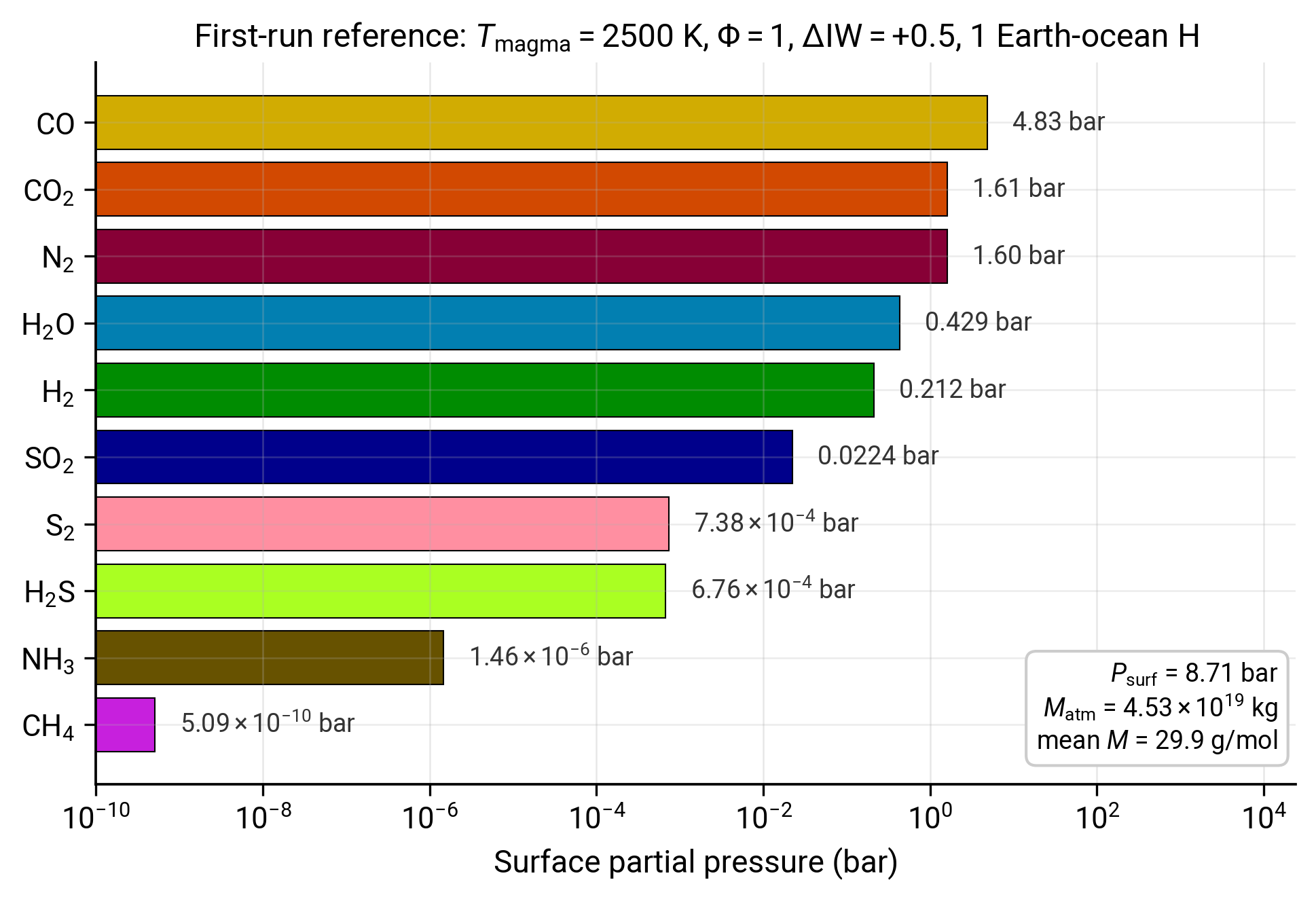
Reference output for the first-run inputs. Species ordered top-to-bottom by partial pressure. The summary box top-right shows the three aggregate diagnostics from Step 3 (\(P_\mathrm{surf}\), \(M_\mathrm{atm}\), mean molar mass).

The five large reservoirs (CO, N\(_2\), CO\(_2\), H\(_2\), H\(_2\)O all between \(\sim 0.2\) and \(\sim 5\) bar) account for essentially the entire \(\sim 9\) bar atmosphere; the four trace species (SO\(_2\), H\(_2\)S, S\(_2\), NH\(_3\)) sit two to seven orders of magnitude lower; CH\(_4\) is effectively absent at this temperature. If your output disagrees by more than a factor of \(\sim 2\) on a major species or by orders of magnitude on the speciation ordering, recheck the ddict keys against the snippet above. The script that produces this reference figure is checked in at scripts/tutorials/fig_firstrun_reference.py and can be re-run with python -m scripts.tutorials.fig_firstrun_reference from the repository root.

Step 6: sweep one parameter

Repeat the solve along a grid of \(\Delta\mathrm{IW}\) to see the redox dependence directly. Reuse the previous solution as the warm start each time:

diw_grid = np.linspace(-5, +5, 21)
p_dict = {sp: [] for sp in species_to_plot}
p_guess = None

for diw in diw_grid:
    ddict['fO2_shift_IW'] = diw
    target = get_target_from_params(ddict)
    result = equilibrium_atmosphere(target, ddict, p_guess=p_guess, print_result=False)
    for sp in species_to_plot:
        p_dict[sp].append(result[f'{sp}_bar'])
    # warm start the next solve with the four primaries
    p_guess = {s: result[f'{s}_bar'] for s in ('H2O', 'CO2', 'N2', 'S2')}

fig, ax = plt.subplots(figsize=(7, 5))
for sp in species_to_plot:
    ax.plot(diw_grid, p_dict[sp], color=dict_colors[sp], label=sp, lw=2)
ax.set_yscale('log')
ax.set_xlabel(r'$\Delta\mathrm{IW}$ ($\log_{10}$ shift from iron-wüstite)')
ax.set_ylabel('Partial pressure (bar)')
ax.set_ylim(1e-6, 1e4)
ax.legend(ncol=2, fontsize=8, loc='best')
ax.grid(which='both', alpha=0.3)
fig.tight_layout()
fig.savefig('redox_sweep.pdf')
plt.show()

The expected qualitative behaviour, consistent with Bower et al. (2022) ¹ Section 3 and Nicholls et al. (2024) ² Figure 6:

• At \(\Delta\mathrm{IW} \le -1\) (reducing), H\(_2\) and CO dominate; H\(_2\)O and CO\(_2\) collapse;
• Around \(\Delta\mathrm{IW} \approx 0\), the H\(_2\)O/H\(_2\) and CO\(_2\)/CO ratios are of order unity;
• At \(\Delta\mathrm{IW} \ge +2\) (oxidising), H\(_2\)O and CO\(_2\) dominate; H\(_2\) and CO are sub-percent.

S\(_2\) stays roughly constant (inventory-controlled), while SO\(_2\) rises and H\(_2\)S falls with increasing \(\Delta\mathrm{IW}\).

Where to go next

• For the equations behind the redox couples, read Equilibrium chemistry.
• For the solubility laws and their references, read Solubility laws.
• For the mass-balance system that ties the partial pressures to the elemental inventory, read Mass balance & solver.
• For the PROTEUS-coupled invocation pattern, read Coupling to PROTEUS (how-to).