Metal reservoir: partition volatiles into the core

This tutorial adds a metal reservoir to a CALLIOPE solve. The metal stands for the liquid iron that forms a planet's core. Some of the H, C, N and S of the melt goes into this metal, so less of it is left for the atmosphere.

By the end of it you will:

have run the same planet without metal and with metal, and compared the results;
know the 2 ways to set the oxygen fugacity of the metal-melt equilibrium (dIW_eq_mode);
know the 2 ways to set the O and Si of the metal (O_mode_core, Si_mode_core), and how to read the FeO exchange;
know what the out-of-range flags and the placeholder warning mean, and what to do about them;
have made a plot of the metal share of each element against \(\Delta\mathrm{IW}\);
have run the authoritative-O solve with metal.

You should already have done the First run tutorial. The physics is on the Metal reservoir explanation page, and every input and output key is on the partition file reference. Run the steps in order in one Python session: each step uses the variables of the steps before it, and the printed numbers below come from that order, with the random start guesses of the solver set once in step 2 (np.random.seed(0)). The whole tutorial runs in less than a minute.

Step 1: the input

Start from the input of the First run tutorial and add the metal keys:

import logging

import matplotlib.pyplot as plt
import numpy as np

from calliope.constants import M_core_earth, volatile_species
from calliope.solve import (
    equilibrium_atmosphere,
    equilibrium_atmosphere_authoritative_O,
    get_target_from_params,
)

logging.basicConfig(level=logging.WARNING, format='%(levelname)s %(message)s')

ddict = {
    # planet and melt, as in the First run tutorial
    'M_mantle': 4.03e24,  # kg
    'gravity': 9.81,  # m s-2
    'radius': 6.371e6,  # m
    'T_magma': 2500.0,  # K
    'Phi_global': 1.0,  # fully molten
    'fO2_shift_IW': 0.5,  # surface gas and melt, relative to the IW buffer
    'hydrogen_earth_oceans': 1.0,
    'CH_ratio': 0.1,
    'nitrogen_ppmw': 2.0,
    'sulfur_ppmw': 200.0,
}
for sp in volatile_species:
    ddict[f'{sp}_included'] = 1
    ddict[f'{sp}_initial_bar'] = 0.0

metal = {
    'metal_mass': M_core_earth,  # kg, the whole Earth core (1.94e24 kg)
    'P_eq': 50.0,  # GPa
    'T_eq': 3500.0,  # K
    'dIW_eq_mode': 'parameter',
    'dIW_eq': -1.0,  # log10 units relative to the IW buffer
}
target = get_target_from_params(ddict)

The metal keys:

metal_mass (kg) is the metal that is in equilibrium with the present melt. Here it is the whole Earth core, in equilibrium with the whole mantle at one pressure and temperature (the single-stage case; the explanation page says why). Any value above 0 turns the metal reservoir on.
P_eq (GPa) and T_eq (K) are the pressure and temperature of the metal-melt equilibrium. They are not the surface values: the metal equilibrates deep in the magma ocean.
dIW_eq (log10 units) is the oxygen fugacity of that equilibrium relative to the iron-wüstite (IW) buffer. It is a separate input from fO2_shift_IW, which sets the gas and the melt at the surface.

The logging line makes the warnings of CALLIOPE visible. The solves of steps 2 to 4 log warnings; step 5 explains each of them.

Step 2: solve without metal and with metal

np.random.seed(0)
no_metal = equilibrium_atmosphere(target, {**ddict, 'metal_mass': 0.0}, print_result=False)
with_metal = equilibrium_atmosphere(target, {**ddict, **metal}, print_result=False)

print(f"P_surf: {no_metal['P_surf']:.3g} bar without metal, {with_metal['P_surf']:.3g} bar with metal")
print('el  D_metal  w_core     kg_core    kg_total   bulk       metal share')
for el in ('H', 'C', 'N', 'S'):
    core, total = with_metal[f'{el}_kg_core'], with_metal[f'{el}_kg_total']
    print(
        f"{el:2s}  {with_metal[f'{el}_D_metal']:<7.4g}  {with_metal[f'w_{el}_core']:.3e}  "
        f'{core:.3e}  {total:.3e}  {core + total:.3e}  {core / (core + total):.4f}'
    )
print('budget: ' + ', '.join(f'{el} {target[el]:.3e}' for el in ('H', 'C', 'N', 'S')))

The output:

P_surf: 8.7 bar without metal, 7.67 bar with metal
el  D_metal  w_core     kg_core    kg_total   bulk       metal share
H   22.14    7.304e-05  1.417e+20  1.330e+19  1.550e+20  0.9142
C   0.08284  4.384e-08  8.505e+16  1.541e+19  1.550e+19  0.0055
N   39       1.733e-06  3.362e+18  4.698e+18  8.060e+18  0.4172
S   173      4.105e-04  7.964e+20  9.565e+18  8.060e+20  0.9881
budget: H 1.550e+20, C 1.550e+19, N 8.060e+18, S 8.060e+20

How to read the columns:

<e>_D_metal is the partition coefficient \(D\) on the mass basis: the mass fraction of the element in the metal divided by that in the melt.
w_<e>_core is the mass fraction of the element in the metal, and <e>_kg_core its mass there, in kg.
<e>_kg_total is the gas plus the melt. It does not include the metal.
The bulk inventory of an element is <e>_kg_total + <e>_kg_core. It equals the budget in target (the last line): no mass is lost or made.
The metal share is the bulk inventory in the metal, <e>_kg_core over the bulk. The keys say core for the metal reservoir.

Most of the H and S goes into the metal, and almost no C. The atmosphere of this planet is mostly CO and CO\(_2\), so the surface pressure falls only from 8.7 to 7.67 bar.

A solve with metal_mass = 0 is the solve without metal. Its result holds <e>_kg_core = 0 for H, C, N and S and none of the other metal keys:

for el in ('H', 'C', 'N', 'S'):
    print(f"{el}: core {no_metal[f'{el}_kg_core']}, D_metal in result: {f'{el}_D_metal' in no_metal}")

H: core 0.0, D_metal in result: False
C: core 0.0, D_metal in result: False
N: core 0.0, D_metal in result: False
S: core 0.0, D_metal in result: False

Step 3: the 2 modes of \(\Delta\mathrm{IW}\)

dIW_eq_mode selects where the \(\Delta\mathrm{IW}\) of the partition laws comes from:

'parameter': from dIW_eq, as in step 2.
'from_FeO': from the FeO of the melt and the Fe of the metal, \(\Delta\mathrm{IW} = 2\log_{10}(x_\mathrm{FeO}/x'_\mathrm{Fe})\). Here \(x_\mathrm{FeO}\) is the mole fraction of FeO in the melt on the single-cation basis, and \(x'_\mathrm{Fe}\) the mole fraction of Fe in the metal without H and C. The melt composition is silicate_oxides, KLB-1 by default.

from_feo = equilibrium_atmosphere(
    target, {**ddict, **metal, 'dIW_eq_mode': 'from_FeO'}, print_result=False
)
for name, res in (('parameter', with_metal), ('from_FeO', from_feo)):
    d_values = ', '.join(f"{el} {res[f'{el}_D_metal']:.3g}" for el in ('H', 'C', 'N', 'S'))
    flags = ''.join(el for el in ('H', 'C', 'N', 'S') if res[f'{el}_D_out_of_range'])
    print(f"{name:9s}  dIW_eq {res['dIW_eq']:+.3f}  D: {d_values}  flagged: {flags}")

parameter  dIW_eq -1.000  D: H 22.1, C 0.0828, N 39, S 173  flagged: NS
from_FeO   dIW_eq -2.484  D: H 52, C 0.187, N 6.37, S 42.2  flagged: HNS

The result gives the \(\Delta\mathrm{IW}\) it used as dIW_eq. With the KLB-1 melt (8.10 wt% FeO) and metal without O and Si, 'from_FeO' gives \(-2.48\). This is outside the range of the H law (\(-1.33\) to \(-0.88\)), so H is flagged as well.

Step 4: O and Si in the metal

O and Si enter the metal by exchange with the silicate: \(\mathrm{FeO} = \mathrm{Fe} + \mathrm{O}\) and \(\mathrm{SiO_2} + 2\,\mathrm{Fe} = \mathrm{Si} + 2\,\mathrm{FeO}\). O_mode_core and Si_mode_core select how CALLIOPE sets them:

'fixed' (default): the metal holds w_O_core and w_Si_core (mass fractions, default 0).
'partition': the exchange coefficients of the partition file and the \(\Delta\mathrm{IW}\) of each pass set them.

fixed = equilibrium_atmosphere(
    target, {**ddict, **metal, 'w_O_core': 0.02, 'w_Si_core': 0.05}, print_result=False
)  # example values, not a model of the Earth's core
partition = equilibrium_atmosphere(
    target,
    {**ddict, **metal, 'O_mode_core': 'partition', 'Si_mode_core': 'partition'},
    print_result=False,
)
for name, res in (('fixed', fixed), ('partition', partition)):
    ratio = res['n_FeO_exchange'] / res['n_FeO_silicate']
    print(
        f"{name:9s}  w_O {res['w_O_core']:.4f}  w_Si {res['w_Si_core']:.4f}  "
        f"n_FeO_exchange {res['n_FeO_exchange']:+.3e} mol ({ratio:+.2f} of the melt FeO)  "
        f"FeO_exchange_out_of_range {res['FeO_exchange_out_of_range']}  "
        f"D_C {res['C_D_metal']:.3g}"
    )
print('O and Si flags in partition mode:', partition['O_D_out_of_range'], partition['Si_D_out_of_range'])

fixed      w_O 0.0200  w_Si 0.0500  n_FeO_exchange -4.482e+24 mol (-0.99 of the melt FeO)  FeO_exchange_out_of_range 1  D_C 0.298
partition  w_O 0.1366  w_Si 0.0027  n_FeO_exchange +1.619e+25 mol (+3.56 of the melt FeO)  FeO_exchange_out_of_range 1  D_C 430
O and Si flags in partition mode: 1 1

How to read the exchange:

n_FeO_exchange (mol) is the FeO that the metal took from the melt: 1 FeO per O atom, minus 2 FeO per Si atom (the Si reaction gives FeO back). A negative value means that the metal gave FeO to the melt.
n_FeO_silicate (mol) is the FeO of the melt.
FeO_exchange_out_of_range is 1 when the exchange is more than 10 % of the melt FeO. CALLIOPE does not change the melt FeO, so such a result is not self-consistent. With the whole core as metal, a few wt% of O or Si already moves a large part of the melt FeO.

In 'partition' mode the metal takes 13.7 wt% O. Net of the Si reaction, the exchange needs 3.56 times the FeO that the melt has, which is not possible. The metal O also enters the C law through its composition term, and \(D_\mathrm{C}\) rises from 0.0828 to 430. The O and Si of the metal come from the FeO of the rock, so they never enter the volatile O budget (see step 7).

Step 5: read the warnings and the flags

The first solves of this tutorial logged these warnings (each one once per process):

WARNING the metal partition laws are placeholders
WARNING N partition law evaluated outside its range or on an unknown range: P_eq 50 GPa, T_eq 3500 K, dIW_eq -1
WARNING S partition law evaluated outside its range or on an unknown range: P_eq 50 GPa, T_eq 3500 K, dIW_eq -1
WARNING H partition law evaluated outside its range or on an unknown range: P_eq 50 GPa, T_eq 3500 K, dIW_eq -2.48
WARNING the metal exchange takes more than 10 % of the silicate FeO (0.987); the melt FeO and dIW_eq of this solve do not follow it
WARNING O_mode_core 'partition' uses ideal activities in metal and melt; activity coefficients are not included
WARNING Si_mode_core 'partition' uses ideal activities in metal and melt; activity coefficients are not included
WARNING O partition law evaluated outside its range or on an unknown range: P_eq 50 GPa, T_eq 3500 K, dIW_eq -1
WARNING Si partition law evaluated outside its range or on an unknown range: P_eq 50 GPa, T_eq 3500 K, dIW_eq -1

What each one means, and what to do:

The laws are placeholders. The packaged partition file has placeholder = true. Its laws come from published values, but some are simple lines through 2 table values. For a result you want to publish, put a fitted law from a source you have read into your own file: see Add a new partition law.
A law outside its range. <e>_D_out_of_range is 1 and the warning names the conditions. The pressure, temperature or \(\Delta\mathrm{IW}\) is outside the data that the law was fitted to, or the range is unknown. The placeholder N and S laws are in range only at one pressure and temperature (N: 20 GPa, 3000 K; S: 60 GPa, 4000 K). The placeholder O and Si laws have no known temperature and \(\Delta\mathrm{IW}\) range, so they are always flagged. With the packaged file, no P_eq and T_eq put N and S in range together, so every result with this file has at least one flag. Use a law whose range covers your conditions (Add a new partition law), or move the conditions into the range of the law you have. If you keep a flagged result, say in your text that the law was extrapolated.
The FeO exchange. More than 10 % of the melt FeO moved. Use less metal O and Si, or apply the exchange to the FeO budget of your own model.
Ideal activities. 'partition' mode leaves out the activity coefficients of the published O and Si fits. Treat its O and Si as a first estimate.

The solve does not stop or clamp a value for any of these: it returns the result with the flags set. The flags are in the result dictionary, so a script can check them; the warnings appear only once per process.

Scan dIW_eq from \(-3\) to 0 and plot the metal share of each element. Each solve starts from the partial pressures of the solve before (p_guess), which makes the scan faster:

d_iw_grid = np.linspace(-3.0, 0.0, 13)
share = {el: [] for el in ('H', 'C', 'N', 'S')}
p_guess = None
for d_iw in d_iw_grid:
    res = equilibrium_atmosphere(
        target, {**ddict, **metal, 'dIW_eq': float(d_iw)}, p_guess=p_guess, print_result=False
    )
    p_guess = {s: res[f'{s}_bar'] for s in ('H2O', 'CO2', 'N2', 'S2')}
    for el in share:
        core = res[f'{el}_kg_core']
        share[el].append(core / (core + res[f'{el}_kg_total']))

fig, ax = plt.subplots(figsize=(6, 4))
for el, style in zip(share, ('o-', 's-', '^--', 'v--')):
    ax.plot(d_iw_grid, share[el], style, label=el)
ax.axvspan(-1.33, -0.88, color='0.85', label='range of the H law')
ax.set_xlabel(r'$\Delta\mathrm{IW}$ of the metal-melt equilibrium (dIW_eq)')
ax.set_ylabel('share of the bulk inventory in the metal')
ax.set_yscale('log')
ax.legend()
fig.tight_layout()
fig.savefig('metal_core_share.png', dpi=150)
for i in (0, 4, 8, 12):
    print(f"dIW_eq {d_iw_grid[i]:+.2f}: " + ', '.join(f'{el} {share[el][i]:.3g}' for el in share))

dIW_eq -3.00: H 0.971, C 0.0162, N 0.057, S 0.926
dIW_eq -2.00: H 0.95, C 0.00942, N 0.171, S 0.97
dIW_eq -1.00: H 0.914, C 0.00549, N 0.417, S 0.988
dIW_eq +0.00: H 0.857, C 0.0032, N 0.718, S 0.995

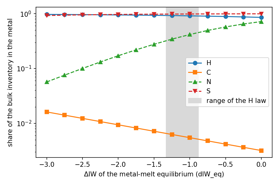
Log plot of the metal share of H, C, N and S against dIW_eq from -3 to 0: H and S near 1, N rising from 0.06 to 0.7, C falling from 0.016 to 0.003

Metal share of the bulk H, C, N and S inventory against dIW_eq, for the whole Earth core at 50 GPa and 3500 K. The y axis is logarithmic. The grey band is the \(\Delta\mathrm{IW}\) range of the placeholder H law; outside it, the H law is out of range. The C law is out of range above \(-0.53\). The N and S laws (dashed) are out of range at every point, because each is in range only at one other pressure and temperature. A solid line does not mean that the law is in range.

How to read the plot:

N goes into the metal more at higher \(\Delta\mathrm{IW}\), because its placeholder law rises with \(\Delta\mathrm{IW}\).
C goes into the metal less at higher \(\Delta\mathrm{IW}\): the C law has a negative \(\Delta\mathrm{IW}\) term. Above \(-0.53\) the C law is out of range too, and a warning names it.
H and S stay above 85 % over the whole scan.

Step 7: the authoritative-O solve with metal

The authoritative-O solve takes the O of the gas and the melt as a budget and finds the oxygen fugacity. With metal, the metal O is not part of this budget, because it comes from the FeO of the rock. Give the metal 0.1 wt% O, solve with the buffer, and give the gas and melt O of that solve back as a budget:

metal_o = {**metal, 'w_O_core': 0.001}  # 0.1 wt% O in the metal
buffered = equilibrium_atmosphere(target, {**ddict, **metal_o}, print_result=False)
o_budget = buffered['O_kg_total']  # gas and melt O

guess = {s: buffered[f'{s}_bar'] for s in ('H2O', 'CO2', 'N2', 'S2')}
guess['fO2_shift_IW'] = ddict['fO2_shift_IW']
auth = equilibrium_atmosphere_authoritative_O(
    {**target, 'O': o_budget}, {**ddict, **metal_o}, p_guess=guess, print_result=False
)
print(f"fO2_shift_derived {auth['fO2_shift_derived']:+.6f} (buffered input {ddict['fO2_shift_IW']:+.1f})")
print(f"O budget {o_budget:.4e} kg, gas + melt O {auth['O_kg_atm'] + auth['O_kg_liquid']:.4e} kg")
print(f"O_kg_core {auth['O_kg_core']:.3e} kg")

fO2_shift_derived +0.500000 (buffered input +0.5)
O budget 1.3129e+20 kg, gas + melt O 1.3129e+20 kg
O_kg_core 1.940e+21 kg

This is a round trip: the O of a buffered solve, given back as a budget, must give back the \(\Delta\mathrm{IW}\) of that buffered solve. The solve returns +0.5, and the gas and melt O equal the budget. The metal holds about 15 times more O than the gas and the melt, and none of it is counted in the budget. The guess p_guess holds the 4 primary partial pressures and fO2_shift_IW; without it, the solve starts from random guesses and took 41 to 63 s here in 3 runs with different random starts, instead of a fraction of a second.

Where to go next

Metal reservoir: the physics, a worked example and the limits.
Add a new partition law: replace a placeholder law with a law from a paper.
Partition file reference: every input and output key and the file format.
Metal reservoir validation: how the tests check the metal reservoir.