Solid-state convection
What this page checks
This page covers the solid-state part of Aragog: the activation law of solid creep, the mixing length below a stagnant lid, the cooling of a mantle under a lid, and how its heat loss scales. The physics is on the Solid-state convection page.
Validation means that we run the code on a case where another source gives the right answer: an analytical result, a published table or a second independent model. We then check that the code gives that answer. If this part of the code were wrong, a standalone Aragog run with rheology.enabled = true would have the wrong mantle temperature, lid thickness and surface heat flux.
Read the known limits. The saturating activation law passes against its references. The top slope, the 0-D comparison and the internal-heating exponents do not meet all their published or derived bounds. For these cases, the tests store the computed values and fail if a later change shifts them. Each Known limit. line states what does not match.
Each case gives, where they apply and in roughly this order: why the check exists, what it tests, how we know the right answer, the setup, the result, why it matters, the plot, a known limit and the test details.
The saturating activation law gives its limits
Why this check exists. A fault in the activation law changes the viscosity of the deep mantle. The test fails if the law loses its linear limit or its isobaric limit, if its derivative is wrong, or if it leaves the Lagrange bound.
What it tests. The saturating integral law gives the activation enthalpy \(H(P)\) from the zero-pressure energy \(E_a\), the zero-pressure volume \(V_0\) and the decay pressure \(P_\text{decay}\). The test compares it with its limits over \(P \in [0, 1000]\text{ GPa}\) in NumPy and JAX.
How we know the right answer. The limits follow from the formula. At \(P_\text{decay} = \infty\) it is the linear activation-volume law of the published papers. At \(V_0 = 0\) it is the isobaric law. For finite \(P_\text{decay}\), Taylor's theorem with the Lagrange remainder gives the bound.
Why it matters. compute_arrhenius_viscosity uses this enthalpy when activation_energy is set, so the law sets the viscosity at depth.
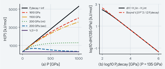
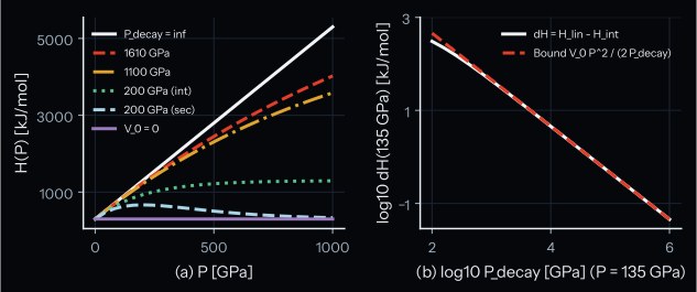
How to read the plot. A pass: in panel (b), \(\mathrm{d}H\) lies on or below the bound. Panel (a) plots \(H(P)\) over pressure \(P \in [0, 1000]\text{ GPa}\) for \(E_a = 300\text{ kJ mol}^{-1}\) and \(V_0 = 5.0\text{ cm}^3\text{ mol}^{-1}\). It compares curves for \(P_\text{decay} \in \{200, 1100, 1610, \infty\}\text{ GPa}\) with the \(P_\text{decay} = 200\text{ GPa}\) secant curve and the \(V_0 = 0\) isobaric limit. Panel (b) plots the enthalpy difference \(\mathrm{d}H = H_\text{lin}(P) - H_\text{int}(P)\) against the analytical Lagrange bound \(\text{Bound} = V_0 P^2 / (2 P_\text{decay})\). The secant curve fails this bound, and the test asserts that it does.
Panel (b) uses Earth core-mantle boundary pressure \(P = 135\text{ GPa}\) over decay pressures \(P_\text{decay} \in [10^2, 10^6]\text{ GPa}\) (\(E_a = 300\text{ kJ mol}^{-1}\), \(V_0 = 5.0\text{ cm}^3\text{ mol}^{-1}\), where \(V_0 P^2 / 2 = 45562.5\text{ kJ mol}^{-1}\text{ GPa}\)). The secant curve is \(E_0 + P V_0 \exp(-P / P_\text{decay})\), the form of the rows of Tackley et al. (2013)9, Table 2, with finite \(P_\text{decay}\).
Test details
- Reference: Linear activation-volume law \(H_\text{lin}(P) = E_a + V_0 P\) of Karato and Wu (1993)4 (p. 772, eq. 1), Armann and Tackley (2012)1 (p. 4, eq. 1: \(E_a = 300\text{ kJ mol}^{-1}\), \(V_0 = 6.0\text{ cm}^3\text{ mol}^{-1}\)), and Tackley et al. (2013)9 (eqs. 2-3 and Table 2 upper-mantle row, pp. 4 and 19 of the accepted manuscript: \(E_0 = 300\text{ kJ mol}^{-1}\), \(V_0 = 5.0\text{ cm}^3\text{ mol}^{-1}\), \(p_\text{decay} = \infty\)), and isobaric limit \(H(P) = E_a\) at \(V_0 = 0\).
- Tolerance: Bitwise equality (
0.0relative,0ulp) for bothcompute_arrhenius_enthalpyandcompute_arrhenius_viscosityat \(P_\text{decay} = \infty\) and at \(V_0 = 0\) over \(P \in [0, 1000]\text{ GPa}\) in both NumPy and JAX;jax.gradderivative \(\partial H / \partial P = V_0 \exp(-P / P_\text{decay})\) to \(10^{-12}\) relative; for finite \(P_\text{decay} > 0\), analytical Lagrange remainder bound \(0 \le \mathrm{d}H(P) = H_\text{lin}(P) - H(P) \le \text{Bound}(P) = V_0 P^2 / (2 P_\text{decay})\) (evaluated over \(P \in [0, 1000]\text{ GPa}\) in panel a and at \(P = 135\text{ GPa}\) over \(P_\text{decay} \in [10^2, 10^6]\text{ GPa}\) in panel b). - Test id:
tests/test_rheology_verification.py::test_saturating_activation_enthalpy_limits - Command:
pytest tests/test_rheology_verification.py -k test_saturating_activation_enthalpy_limits(add--validation-plotsto write the plot pair)
The top slope against published convection grids
Why this check exists. The top slope \(s_\text{top}(\theta)\) represents how a cold, high-viscosity lid shortens the mixing length, where \(\theta\) is the viscosity-contrast parameter. It reduces the convective flux over most of the depth. The stored evaluation shows how far one slope law reproduces 2 published sets of convection runs.
What it tests. Aragog runs to steady state for each published case, with the slope fixed at the \(\theta\) of that case. The result is compared with the published value. tests/reference/ssc_mlt_top_slope_calibration.json holds the results for 2 slope pairs \((s_{\text{top},\infty}, c_\theta)\):
- The model default, \((0.22, 0.15)\). This is the pair that a run uses unless it sets another one.
- The second pair, \((0.25, 0.25)\). This pair was chosen on these benchmark rows, and the file labels it
minimax_0p25_0p25. The 0-D and scaling-exponent cases below also use it. It is not the code default.
python tools/verification/evaluate_mlt_top_slope_calibration.py --full generates the file, and --check recomputes E340 and f60_H4 live and verifies all stored rows and summary statistics. A label such as E340 is a row of Korenaga (2009)5, Table 1, named for its activation energy in kJ/mol. A label such as f70_1e7_H2 is a row of Deschamps and Vilella (2021)2, Table 1, named for its radius ratio (0.70), its viscosity contrast (\(10^7\)) and its heating (\(H = 2\)). A label such as f80_32_1e6_H4 also gives the Rayleigh-number entry (32).
How we know the right answer. The references are published convection experiments, and each has a tolerance on the compared quantity.
| Benchmark | Grid | Observables and tolerance |
|---|---|---|
| Planar internally heated Newtonian stagnant-lid convection: Korenaga (2009)5, Table 1, the 12 cases with \(n = 1\) | \(N = 100\) uniform planar Boussinesq | Nusselt number \(\mathrm{Nu}\), \(10\%\) relative; \(r_\text{norm} = \lvert\mathrm{Nu} - \mathrm{Nu}_\text{ref}\rvert / (0.10 \, \mathrm{Nu}_\text{ref})\) |
| Spherical mixed-heating stagnant-lid convection: Deschamps and Vilella (2021)2, Table 1, 24 of the 25 spherical cases, 72 observables | \(N = 100\) spherical-shell Boussinesq; \(f = r_\text{in} / r_\text{out} \in \{0.60, 0.70, 0.75, 0.80, 0.85\}\) | Interior temperature \(T_m\), \(0.03\) absolute; top heat flow \(\Phi_\text{top}\), \(15\%\) relative; lid thickness \(d_\text{lid}\), \(20\%\) relative |
Two spherical entries of that table print the same parameters, \(Ra_\text{surf} = 10\), \(f = 0.70\), \(\Delta\eta = 10^6\), \(\tilde{H} = 8\), with different grids and results: \(T_m\) 1.035 and \(\Phi_\text{top}\) 5.596 at \(256 \times 768 \times 128 \times 2\), and \(T_m\) 0.964 and \(\Phi_\text{top}\) 3.964 at \(192 \times 576 \times 96 \times 2\). The row f70_1e6_H8 uses the first and the second is left out. The second lies near the entry with \(\tilde{H} = 4\) at \(f = 0.80\) (\(T_m\) 0.977, \(\Phi_\text{top}\) 4.267), so its \(\tilde{H}\) may be a misprint; the paper does not say.
Setup.
stress_closure_mode = 'local', with \(s_\text{top}\) frozen at the nominal \(\theta\) of each table throughc_theta = 0.- The prescribed surface temperature of the solver (
outer_boundary_condition = 5). - A half-cell conductive boundary-flux patch on inner boundary condition (BC) 3 through
_patched_state_update. - A Frank-Kamenetskii viscosity override during steady-state integration on the spherical cases.
Results. The test recomputes E340 and f60_H4 live, checks the other stored rows and the summary values for consistency, and fails on a difference. It does not assert agreement with the published values.
| Result | Second pair \((0.25, 0.25)\) | Default pair \((0.22, 0.15)\) |
|---|---|---|
| Korenaga cases outside \(10\%\) | \(0\) of \(12\) | \(12\) of \(12\) |
| Largest \(\max \lvert r_\text{norm} \rvert\) | \(0.9839\) on E340 (\(\mathrm{Nu} = 3.3391\) against \(\mathrm{Nu}_\text{ref} = 3.04\), \(+9.84\%\)) |
\(1.4062\) on E210 |
| \(J_\text{Korenaga}\) (mean-square normalized residual) | \(0.8923\) | \(1.3883\) |
| Spherical residuals above \(1.0\) | \(34\) of \(72\) | \(42\) of \(72\) |
| Worst \(r_\Phi\) | \(\max \lvert r_\Phi \rvert = 2.1909\) on f70_1e7_H2 (\(r_\Phi = -2.1909\)) |
\(\max \lvert r_\Phi \rvert = 2.0141\) on f70_1e7_H2 |
| Worst \(r_{T_m}\) | \(\max \lvert r_{T_m} \rvert = 1.9421\) on f80_H2 (\(r_{T_m} = -1.9421\)) |
\(\max \lvert r_{T_m} \rvert = 2.4116\) on f80_H2 |
| Worst \(r_d\) | \(\max \lvert r_d \rvert = 1.3195\) on f80_10_1e6_H10 (\(r_d = -1.3195\)) |
\(\max \lvert r_d \rvert = 1.5597\) on f85_10_1e6_H8 |
| \(J_\text{DV}\) | \(1.0570\) | \(1.4659\) |
| \(J_\text{all}\) over all \(84\) observables (\(36\) total cases) | \(1.0334\) | \(1.4549\) |
On the Korenaga rows, every residual has the same sign: \(\mathrm{Nu}\) is too high in all 12 rows, by \(9.2\) to \(9.8\%\) for the second pair and by \(10.3\) to \(14.1\%\) for the default pair.
Why it matters. In 'lid' mode, pass 2 of the solver passes \(\theta\) to the mixing-length factor, so the slope acts on the convective flux over most of the depth. These runs use 'local' mode and test the slope at a frozen \(\theta\).
This case has no plot, because its tests check a stored file and hand values and write no plot pair.
Known limit. The default pair misses all 12 planar rows of Korenaga (2009)5, Table 1. The second pair is within the \(10\%\) \(\mathrm{Nu}\) tolerance (\(\max |r_\text{norm}| = 0.9839\)), with local closure and \(s_\text{top}\) frozen at the tabulated \(\theta\). This pair was chosen on the benchmark rows, with all these residuals of one sign, so this is not independent agreement.
The second pair does not satisfy the spherical suite of Deschamps and Vilella (2021)2, Table 1, where \(34\) of \(72\) observables exceed their tolerances (\(0.03\) on \(T_m\), \(15\%\) on \(\Phi_\text{top}\), \(20\%\) on \(d_\text{lid}\)). The pair was chosen on these rows too, so these misses remain after the choice.
A single contrast-dependent upper slope \(s_\text{top}(\theta)\) without a spherical-curvature geometry factor cannot match both planar internally heated and spherical mixed-heating stagnant-lid scaling across core-to-planet radius ratios \(f \in [0.60, 0.85]\).
Test details
- Reference: Korenaga (2009)5, Table 1; Deschamps and Vilella (2021)2, Table 1. Hand values and limits of the slope at the default pair: \(s_\text{top}(\theta \le 0) = 1.0\), \(s_\text{top}(15) = 0.3022113951582542\).
- Tolerance:
--checkof the stored file; hand values and limits 1e-15 to 1e-13 relative. The--checktest also runs the 0-D, scaling-exponent and solver-wiring generators (the solver-wiring check is skipped without the SPIDER P-S tables). It checks the stored file and does not assert agreement with the published values. The hand-value test is thereference_pinnedtest. - Test id:
tests/test_mlt_calibration_smoke.py::test_benchmark_generators_check_mode_passes_on_committed_jsons(stored file);tests/test_mlt_calibration.py::test_theta_dependent_top_slope_hand_values_and_limits(hand values) - Command:
pytest tests/test_mlt_calibration_smoke.py -k test_benchmark_generators_check_mode_passes_on_committed_jsons;pytest tests/test_mlt_calibration.py -k test_theta_dependent_top_slope_hand_values_and_limits;python tools/verification/evaluate_mlt_top_slope_calibration.py --check
The 1-D solver against a 0-D cooling model
Why this check exists. Planetary thermal-history models often use a zero-dimensional (0-D) energy balance, an ordinary differential equation (ODE), to estimate interior cooling and lid growth. If the lid geometry, the mixing-length slope or the plastic yield blend of the one-dimensional (1-D) solver were miswired, the model would predict the wrong mantle cooling rate or silently ignore yielding. The test fails on these faults:
- Loss of plastic yield in the lid. In
E300at \(N = 100\) and \(\tau_{y,0} = 0.5\,\tau_{d,\text{lid}}\) with fixed internal heating, the test requires at least \(40\) yielding basic nodes (stored \(46\)), and a steady-state entropy residual \(\max |\mathrm{d}S/\mathrm{d}t|\) of at most \(10^{-9}\text{ J kg}^{-1}\text{ K}^{-1}\text{ yr}^{-1}\).E300is the row of Korenaga (2009)5, Table 1, with activation energy \(300\text{ kJ/mol}\);E340andE270are named in the same way. - A change of the top-slope asymptote or the lid-base contrast. The test pins the 1-D lid thickness and the convective flux of the live right-hand side to \(10^{-7}\) relative.
- A change of the 0-D Nusselt prefactor or a parameter default. The test pins the 0-D interior temperature trajectory to \(10^{-7}\) relative. Parity tests assert that the default constants in
tests/reference/stagnant_lid_0d.pymatch theSolidRheologyParamsdefaults insrc/aragog/rheology.py.
What it tests. The radial finite-volume solver EntropySolver against the standalone 0-D stagnant-lid ODE in tests/reference/stagnant_lid_0d.py, over \(4.50\text{ Gyr}\) of secular cooling and in steady-state plastic yield-thinning sweeps. tests/reference/ssc_0d_reference_benchmarks.json holds the results (regenerated with python tools/verification/generate_ssc_0d_reference_benchmarks.py --full and verified with --check). Yield acts only with rheology.enabled = true (default false).
How we know the right answer. The reference trajectory comes from integrating the 0-D stagnant-lid global energy balance with published Nusselt-Rayleigh scaling laws from Korenaga (2009)5 and Solomatov and Moresi (2000)8. The analytical yield-thinning reference \(R_\text{thin,0D} = \min\big(1, (\tau_{y,0} / \tau_{d,\text{lid}})^{1/3}\big)\) follows from a balance of plastic yield stress against convective boundary-layer stress (Moresi and Solomatov, 19986; Foley and Bercovici, 20143). stagnant_lid_0d.py integrates a separate ODE without calling EntropySolver.
Symbols.
| Symbol | Meaning | Unit |
|---|---|---|
| \(T_i\) | Sub-lid interior temperature | \(\text{K}\) |
| \(d_\text{lid}\) | Conductive stagnant-lid thickness | \(\text{m}\) or \(\text{km}\) |
| \(F_\text{top}\) | Surface conductive heat flux | \(\text{W m}^{-2}\) |
| \(\mathrm{Nu}\) | Nusselt number: ratio of total surface heat loss to basal-to-surface conductive heat loss | dimensionless |
| \(\mathrm{Ra}_i\) | Internal Rayleigh number at the interior viscosity \(\eta(T_i, P_i)\) | dimensionless |
| \(\theta\) | Frank-Kamenetskii viscosity-contrast parameter across \(T_i - T_\text{surf}\) | dimensionless |
| \(\tau_{d,\text{lid}}\) | Convective driving stress at the lid base | \(\text{Pa}\) |
| \(\tau_{y,0}\) | Surface yield-stress cohesion ceiling | \(\text{Pa}\) |
| \(R_\text{thin} = d_\text{lid}(\tau_{y,0}) / d_\text{lid}(\text{unyielded})\) | Lid-thinning ratio when plastic yielding is active | dimensionless |
| \(a_\text{lid}\) | Lid contrast coefficient, lid_contrast_coeff |
dimensionless |
| Pass-1 lid | Lid thickness from the isotherm \(T_\text{lid,iso}\) of solver pass 1 | \(\text{km}\) |
| \(D\) | Mantle thickness | \(\text{m}\) |
The prefactors. In the 0-D ODE, \(a_\text{Nu} = 0.5954\) is the arithmetic mean of \(a_\text{Nu} = \mathrm{Nu}_\text{ref}\,\theta^{4/3}\,\mathrm{Ra}_i^{-1/3}\) over the 12 Newtonian Arrhenius 2-D stagnant-lid runs of Korenaga (2009)5, p. 157, Table 1 (\(\min = 0.5025\), \(\max = 0.6862\), standard deviation \(0.0651\); a_nu_provenance in tests/reference/ssc_0d_reference_benchmarks.json). The test also runs 2 published prefactors. The \(0.53\) prefactor of Solomatov and Moresi (2000)8 does not use the Korenaga rows, so that check does not depend on them.
| Prefactor | Source | \(T_{i,\text{0D}}(4.50\text{ Gyr})\) | Largest \(T_i\) deviation at \(4.50\text{ Gyr}\) | On the pre-clamp window \(t < 3.6958\text{ Gyr}\) | Post-relaxation \(d_\text{lid}\) deviation |
|---|---|---|---|---|---|
| \(a_\text{Nu} = 0.53\) | Solomatov and Moresi (2000)8, p. 21803, Table 6; p. 21804, eq. 23 | \(1329.8\text{ K}\) | \(7.78\%\) | \(6.52\%\) | \(46.97\%\) pre-clamp and full-run |
| \(a_\text{Nu} = 0.57\) | Korenaga (2009)5, p. 158, eq. 29; p. 159, Fig. 4a | \(1320.9\text{ K}\) | \(7.16\%\) | \(5.89\%\) | \(46.94\%\) pre-clamp |
The \(a_\text{Nu} = 0.53\) run gives \(d_{\text{lid,0D}}(4.50\text{ Gyr}) = 899.2\text{ km}\).
Setup.
- Material properties are constant in both cases (
eos_method = 1,const_properties = True, no equation-of-state table read). - The steady-state
E300runs prescribe the surface temperature (outer_boundary_condition = 5). The solver sets the surface node to the entropy whose temperature is \(T_\text{surf} = 273.0\text{ K}\) and takes the surface gradient from the half-cell temperature gradient. The top conductive heat flux is then \(F_\text{top} = k (T_\text{cell} - T_\text{surf}) / (\Delta r / 2)\), and the lid closure reads \(T_\text{surf}\).test_rheology_verification_smoke.pyevaluates the storedE300steady states with the same surface temperature. - The \(400\text{ Myr}\) and \(4.50\text{ Gyr}\) secular-cooling trajectories use
outer_boundary_condition = 1(grey-body radiative boundary condition with emissivity \(\varepsilon = 1\) and equilibrium temperature \(T_\text{eq} = 300\text{ K}\)), in a single continuous integration over \([0, t_\text{end}]\).
What the generator does in --full and --check mode
--full. tools/verification/generate_ssc_0d_reference_benchmarks.py temporarily replaces EntropySolver._solve_cvode with an unbounded-step wrapper (max_step = np.inf). This integrates the multi-Gyr trajectories without a stop at the \(100\text{ yr}\) phase-boundary step cap, because the solver caps steps at \(100\text{ yr}\) after solidification.
The tool does not compute the 1-D values of the fixed-input blocks (steady_yield_thinning, live_yield_states, yield_sweep_reference_state, yield_sweep_1d_by_dt, yield_sweep_1d_equal_Ti_from_S_ref, yield_sweep_1d_equal_Ti_1600K_from_init and segment_25Myr_spread_5starts). It reads them from the stored benchmark file, so --full refuses to run without that file.
--check recomputes live: all four 0-D ODE trajectories; a_nu_provenance; yield_sweep_0d_at_1600K; the 0-D fixed-\(T_i\) and fixed-\(H\) yield-thinning ratios; the 1-D segment_25Myr_spread_5starts trajectory integration; the 1-D 10Myr yield integration for unyielded_500MPa and below_0p5x_tau_d_lid; and EntropySolver._dSdt_single on the four endpoint_states profiles, the five 0Myr live_yield_states profiles and the three E300 steady_yield_thinning profiles.
--check also checks: the stored five-start spread statistics in segment_25Myr_spread_5starts satisfy \(0 < \text{spread} < 10^{-7}\) (bounded, not recomputed from the five perturbed starts). The remaining stored 1-D trajectory points, the 5Myr, 20Myr, 30Myr and yield_sweep_1d_equal_Ti yield horizons, and the remaining E300, E340 and E270 steady-state rows are checked for internal algebraic consistency.
Secular cooling over 4.5 Gyr
Setup. The run cools the constant-property spherical mantle of cfg/abe_solid.toml from \(T_\text{init} = 1800\text{ K}\) to \(4.50\text{ Gyr}\) at \((s_{\text{top},\infty}, c_\theta) = (0.25, 0.25)\).
| Parameter | Value |
|---|---|
| Radii, mesh | \(r_\text{out} = 6371\text{ km}\), \(r_\text{in} = 5371\text{ km}\), \(N = 100\) |
| Density, specific heat capacity | \(\rho = 4200\text{ kg m}^{-3}\), \(c_p = 1000\text{ J kg}^{-1}\text{ K}^{-1}\) |
| Thermal expansivity, conductivity | \(\alpha = 1 \times 10^{-5}\text{ K}^{-1}\), \(k = 4.0\text{ W m}^{-1}\text{ K}^{-1}\) |
| Reference interior pressure, solid viscosity | \(P_i = 4.1202\text{ GPa}\), \(\eta_\text{solid} = 10^{18}\text{ Pa s}\) |
| Homologous exponent | \(g_\text{hom} = 25.0\) |
| Boundaries | \(T_\text{surf} = 300\text{ K}\), \(F_\text{bot} = 0\) |
| Unyielded yield stress | \(\tau_y = 500\text{ MPa}\) |
The 0-D model. It integrates \(-c_\text{eff}\,\mathrm{d}T_i/\mathrm{d}t = 4\pi r_\text{out}^2 F_\text{top}\) with bulk heat capacity \(c_\text{eff} = m_\text{mantle} c_p\) over the whole spherical shell. The whole mantle cools at the single rate \(\mathrm{d}T_i/\mathrm{d}t\), and no radial profile \(T(r, t)\) evolves. It clamps \(\mathrm{Nu} = \max(\mathrm{Nu}_\text{unyielded}, 1.0)\). It scales the spherical surface heat flux by the conductive shell factor \((r_\text{out} - \delta_{l,\text{eff}}) / r_\text{out}\) at the total thermal boundary-layer thickness \(\delta_{l,\text{eff}} = d_\text{lid,eff} / (1 - a_\text{lid}/\theta)\).
The validity window of the 0-D model. Along its trajectory (\(a_\text{Nu} = 0.5954\)), \(\mathrm{Nu}_\text{unyielded}\) decreases from \(16.328\) at \(t = 0\text{ yr}\) to below \(1.0\) at \(t = 3.6958\text{ Gyr}\) (\(\mathrm{Nu}_\text{unyielded}(3.6324\text{ Gyr}) = 1.0074\) and \(\mathrm{Nu}_\text{unyielded}(3.6958\text{ Gyr}) = 0.9917\), then \(0.8121\) at \(4.50\text{ Gyr}\)).
After the \(\mathrm{Nu} = 1.0\) clamp activates at \(3.6958\text{ Gyr}\), the 0-D lid follows \(d_\text{lid,0D} = (1 - a_\text{lid}/\theta)\,D / \mathrm{Nu} = (1 - 2.2/\theta)\,D\). It rises from \(898.62\text{ km}\) at \(3.6958\text{ Gyr}\) (\(\theta = 21.70\); up from \(891.89\text{ km}\) at \(3.6324\text{ Gyr}\)) to \(899.94\text{ km}\) at \(4.50\text{ Gyr}\) (\(\theta = 21.99\)).
Deviation from the 0-D model.
| Quantity | Interval | Relative deviation |
|---|---|---|
| Lid, post-relaxation (\(t \ge 25\text{ Myr}\)) | Strict window \(\mathrm{Nu}_\text{unyielded} > 1\) (\(t < 3.6958\text{ Gyr}\)) | Reaches \(46.93\%\) at \(3.6324\text{ Gyr}\); crosses the \(22\%\) bound at \(413.0\text{ Myr}\) |
| Lid | \(3.6958\text{ Gyr}\) clamp sample | \(46.73\%\) |
| Lid | \(25\text{ to }400\text{ Myr}\) | \(21.61\%\) |
| Lid | \(t = 0\text{ yr}\), before boundary-layer relaxation | \(100.0\%\) |
| \(T_i\), \(\lvert T_{i,\text{1D}} - T_{i,\text{0D}} \rvert / T_{i,\text{0D}}\) | Crossing of the \(5\%\) bound | \(3.2692\text{ Gyr}\) by linear interpolation; \(3.3234\text{ Gyr}\) at the first grid sample above \(5\%\), where the error is \(5.07\%\) |
| \(T_i\) | Inside the valid window | Reaches \(5.51\%\) at \(3.6324\text{ Gyr}\) |
| \(T_i\) | \(3.6958\text{ Gyr}\) clamp sample | \(5.60\%\) |
| \(T_i\) | \(4.50\text{ Gyr}\) | \(6.78\%\) (\(T_{i,\text{1D}} = 1226.4\text{ K}\) against \(T_{i,\text{0D}} = 1315.6\text{ K}\)) |
| \(T_i\) | \(25\text{ to }400\text{ Myr}\) | Within \(3.61\%\) |
| \(T_i\), default pair \((0.22, 0.15)\) | Full run | \(5.97\%\) |
| Lid, post-relaxation, default pair \((0.22, 0.15)\) | Full run | \(45.28\%\) |
The sign of the offset. At all 128 post-initial samples, the 1-D interior \(T_{i,\text{1D}}(t)\) is cooler than \(T_{i,\text{0D}}(t)\), and the 1-D Pass-1 isotherm lid \(d_{\text{lid,1D}}(t)\) is thinner than \(d_{\text{lid,0D}}(t)\). The lid is \(540.90\text{ km}\) against \(899.94\text{ km}\) at \(4.50\text{ Gyr}\), and \(478.69\text{ km}\) against \(898.62\text{ km}\) at \(3.6958\text{ Gyr}\). The 1-D surface heat flux is higher (\(F_{\text{top,1D}} / F_{\text{top,0D}} = 2.207\) at \(4.50\text{ Gyr}\), \(7.56\text{ mW m}^{-2}\) against \(3.42\text{ mW m}^{-2}\)).
The offset can come from the resolved radial temperature profile across the thickening shell, or from the 1-D spherical mixing-length flux. The cause has not been tested.
Steady-state yield-ceiling lid thinning
Setup. The planar internally heated steady state E300 at \(N = 100\) and \((s_{\text{top},\infty}, c_\theta) = (0.25, 0.25)\). Its unyielded state has \(T_i = 1666.43\text{ K}\), Pass-1 isotherm \(d_\text{lid} = 282.37\text{ km}\), Pass-2 fixed-isotherm depth \(435.21\text{ km}\), \(F_\text{top} = 2078.91\text{ mW m}^{-2}\) and lid driving stress \(\tau_{d,\text{lid}} = 1.956\text{ MPa}\).
How the solver yields. In the two-pass update, the first pass locates \(r_\text{lid,base}\) from the unyielded convective flux fraction and the rheological isotherm \(T_\text{lid,iso} = T_i - 2.2\,\Delta T_\text{rh}\). The second pass lowers \(\eta_\text{eff}\) in the lid and mobilises convective heat transport below \(20.20\text{ km}\) depth (\(20202.02\text{ m} = 2 \times 10^6\text{ m} / 99\), equal to \(2\) radial node spacings on the \(N = 100\) mesh).
Result. At a fixed interior temperature, the 0-D scaling predicts \(R_\text{thin,0D} = \min\big(1, (\tau_{y,0} / \tau_{d,\text{lid}})^{1/3}\big)\). The lid does not thin when the yield stress is above the driving stress, so the value is \(1.0000\) at \(\tau_{y,0} / \tau_{d,\text{lid}} = 2.0\).
At fixed internal heating, the surface flux at steady state balances the heating, so it stays at \(2078.91\text{ mW m}^{-2}\) for every yield stress. With yielding, the 0-D model also carries this flux at a lower interior temperature (\(1631.58\text{ K}\) at \(0.5\,\tau_{d,\text{lid}}\)). At fixed flux its lid scales about with \(T_i - T_\text{surf}\), so its target thins only to \(0.9773\). The solver gives 2 lid measures: Pass-1, the isotherm depth of solver pass 1, and the conductive diagnostic \(d_\text{lid,cond} = (1 - 2.2 / \theta) k (T_i - T_\text{surf}) / F_\text{top}\). The conductive diagnostic comes from the stored fields and is not the solver d_lid output.
At fixed internal heating.
| Quantity | \(\tau_{y,0} / \tau_{d,\text{lid}} = 0.5\) | \(\tau_{y,0} / \tau_{d,\text{lid}} = 0.2\) | \(\tau_{y,0} / \tau_{d,\text{lid}} = 0.1\) |
|---|---|---|---|
| 0-D target at fixed heating | \(0.9773\) | \(0.9482\) | \(0.9270\) |
| Interior temperature | \(1557.05\text{ K}\) | \(1517.88\text{ K}\) | \(1486.01\text{ K}\) |
| Pass-1 isotherm ratio \(R_\text{thin,iso}\) | \(1.5257\), \(+56.1\%\) | \(1.7395\), \(+83.5\%\) | \(1.9116\), \(+106.2\%\) |
| Pass-2 fixed-isotherm depth | \(659.29\text{ km}\) | \(491.18\text{ km}\) | \(468.59\text{ km}\) |
| Same, as a ratio to \(435.21\text{ km}\) | \(1.5149\) | \(1.1286\) | \(1.0767\) |
| Conductive diagnostic ratio | \(0.9282\), \(-5.0\%\) | \(0.9022\), \(-4.9\%\) | \(0.8809\), \(-5.0\%\) |
At the matched interior temperature \(T_i = 1666.43\text{ K}\).
| Quantity | \(\tau_{y,0} / \tau_{d,\text{lid}} = 0.5\) | \(\tau_{y,0} / \tau_{d,\text{lid}} = 0.2\) | \(\tau_{y,0} / \tau_{d,\text{lid}} = 0.1\) |
|---|---|---|---|
| 0-D target \(R_\text{thin,0D}\) | \(0.7937\) | \(0.5848\) | \(0.4642\) |
| Top flux \(F_\text{top}\) (\(\text{mW m}^{-2}\)) | \(3407.08\) | \(4168.05\) | \(4941.39\) |
| Pass-1 isotherm ratio | \(1.0465\), \(+31.9\%\) | \(1.0549\), \(+80.4\%\) | \(1.0578\), \(+127.9\%\) |
| Pass-2 fixed-isotherm depth | \(392.63\text{ km}\) | \(225.93\text{ km}\) | \(179.61\text{ km}\) |
| Same, as a ratio to \(435.21\text{ km}\) | \(0.9022\) | \(0.5191\) | \(0.4127\) |
| Conductive diagnostic ratio | \(0.6102\), \(-23.1\%\) | \(0.4988\), \(-14.7\%\) | \(0.4207\), \(-9.4\%\) |
Percentages are the difference from the 0-D target of the same table.
Against the \(11\%\) relative bound, the Pass-1 ratio fails in both tables: the Pass-1 lid thickens, while the 0-D model predicts that it thins. At the matched \(T_i\) the conductive diagnostic fails at \(0.5\) and \(0.2\,\tau_{d,\text{lid}}\), and it lies within \(11\%\) only at \(0.1\,\tau_{d,\text{lid}}\). At fixed heating, the stored conductive diagnostic lies about \(5\%\) from the fixed-heating target. This is a stored value: no test holds a bound on it, and the --check of the generator recomputes the target. Against the cube-root target, the same values at fixed heating deviate by \(+16.9\%\), \(+54.3\%\) and \(+89.8\%\), and they fail the \(11\%\) bound.
Why it matters. Lid thickness and plastic yielding control how fast a solid rocky mantle loses heat after magma-ocean solidification. They also decide whether lithospheric failure can move a stagnant lid toward mobile-lid cooling in standalone runs.
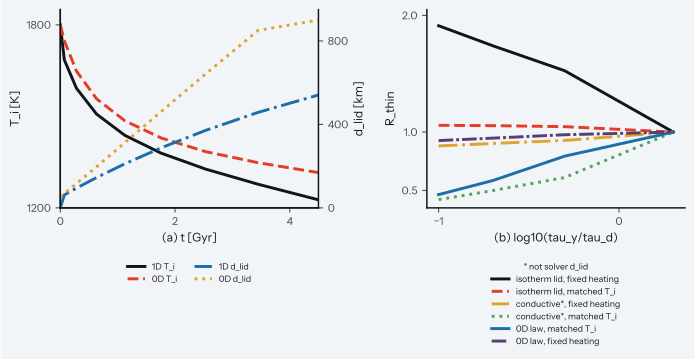
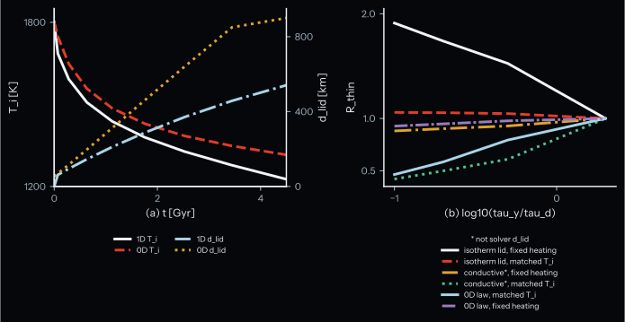
Figure: Comparison of 1-D radial stagnant-lid cooling (panel a) and steady-state yield-thinning ratios (panel b) against the 0-D boundary-layer reference model.
How to read the plot. Panel (a) plots interior temperature \(T_i\) in kelvins (left axis, solid and dashed lines) and lid thickness \(d_\text{lid}\) in kilometres (right axis, dash-dotted and dotted lines) against time in gigayears over \(4.50\text{ Gyr}\). The 1-D lid stays thinner and the 1-D interior cools faster than the 0-D ODE. The 0-D lid follows \((1 - 2.2/\theta)\,D\) from \(898.62\text{ km}\) at \(3.6958\text{ Gyr}\) to \(899.94\text{ km}\) at \(4.50\text{ Gyr}\) once the \(\mathrm{Nu} = 1.0\) clamp engages.
Panel (b) plots the lid-thinning ratio \(R_\text{thin}\) against \(\log_{10}(\tau_{y,0} / \tau_{d,\text{lid}})\). The 2 lines of the 0-D law are the cube-root reference at the matched \(T_i\) and the weaker target at fixed heating. Both decrease as the yield stress drops. The 1-D Pass-1 isotherm ratio stays above \(1.0\), and only the conductive diagnostic thins toward these lines. The star marks the conductive diagnostic, which is not the solver d_lid.
Known limit. The 1-D solver fails the derived 0-D bounds on the \(4.50\text{ Gyr}\) cooling trajectory: \(6.78\%\) full-run and \(5.51\%\) pre-clamp against \(5\%\) on \(T_i\), and \(46.93\%\) pre-clamp and full-run against \(22\%\) on post-relaxation \(d_\text{lid}\). It also fails on the steady-state Pass-1 isotherm yield-thinning ratio: at \(\tau_{y,0} = 0.5\,\tau_{d,\text{lid}}\), \(1.5257\) against the fixed-heating target \(0.9773\) (and against the cube-root target \(0.7937\)), and \(1.0465\) against \(0.7937\) at the matched \(T_i\).
This is consistent with differences between 1-D resolved radial heat transport and the 0-D bulk energy balance, and with plastic yielding that lets convection carry heat only below the top two radial nodes (\(20.20\text{ km}\) depth). The test pins the current 1-D and 0-D values to \(10^{-7}\) relative.
Limit of independence. The 0-D prefactor \(a_\text{Nu} = 0.5954\) is a mean over the 12 Newtonian (\(n = 1\)) rows of Korenaga (2009)5, p. 157, Table 1, and the top-slope pair \((0.25, 0.25)\) was chosen on benchmark rows that include them. A systematic bias in those 12 rows affects both models, and this comparison does not catch it.
Test details
- Reference: Zero-dimensional stagnant-lid energy-balance ODE (
tests/reference/stagnant_lid_0d.py, \(a_\text{Nu}\) =0.5954345503010264), Korenaga (2009)5, p. 157, Table 1; p. 158, eq. 29; p. 159, Fig. 4a, Solomatov and Moresi (2000)8, p. 21803, Table 6; p. 21804, eq. 23, Moresi and Solomatov (1998)6, p. 672, eqs. 11, 13-14; p. 677, eqs. 25-26, and Foley and Bercovici (2014)3, p. 588, eqs. 26-27. - Tolerance: Pinned to
1e-07relative for deterministic single-process evaluation, and1e-07relative on the live \(25\text{ Myr}\) 1-D trajectory segment from its measured 5-start round-off spread (\(\le 4.28 \times 10^{-9}\) on \(T_i\), \(\le 5.25 \times 10^{-9}\) on \(d_\text{lid}\), and \(\le 2.77 \times 10^{-8}\) on \(F_\text{top}\); the comparison fails the derived \(5\%\) \(T_i\), \(22\%\) \(d_\text{lid}\), and \(11\%\) isotherm thinning bounds as documented above). - Test id:
tests/test_rheology_verification_smoke.py::test_0d_stagnant_lid_reference_and_yield_thinning - Command:
pytest tests/test_rheology_verification_smoke.py -k test_0d_stagnant_lid_reference_and_yield_thinning(add--validation-plotsto write the plot pair; regenerate the benchmark file withpython tools/verification/generate_ssc_0d_reference_benchmarks.py --full)
Internal-heating scaling exponents
Why this check exists. If the top-slope formula, the steady-state convective flux or the sub-lid interior temperature diagnostic changed, the scaling of mantle heat loss with radiogenic heating and viscosity contrast would shift silently. The test fails on these faults:
- A change of the top-slope asymptote on steady profiles. The test pins the peak convective heat flux of the steady-state snapshot
case_03(\(\mathrm{Ra}_i = 10^7\), \(\theta = 15\), \(j_\text{conv,max} = 0.8229\text{ W m}^{-2}\)) to \(10^{-7}\) relative. It requires a steady-state entropy residual \(\max |\mathrm{d}S/\mathrm{d}t|\) of at most \(10^{-9}\text{ J kg}^{-1}\text{ K}^{-1}\text{ yr}^{-1}\) (stored \(3.388 \times 10^{-11}\text{ J kg}^{-1}\text{ K}^{-1}\text{ yr}^{-1}\)). - A change of the Nusselt numbers or the regression. The test pins the fitted exponents to \(10^{-7}\) relative.
- Non-convergence of the interior temperature solver.
korenaga_ti_fixed_point(tools/verification/_ssc_helpers.py), the fixed-point solver for the sub-lid temperature of Korenaga (2009)5, p. 156, eq. 20, raisesRuntimeErrorif the iteration does not converge within100steps.
What it tests. In a stagnant-lid mantle heated from within by radioactive decay, boundary-layer theory and two-dimensional (2-D) convection simulations predict a power law for the Nusselt number: \(\mathrm{Nu} = a\,\theta^{-\alpha}\,\mathrm{Ra}_i^\beta\) with \(\beta \approx 1/3\) and \(\alpha \approx 4/3\). The test runs the 1-D viscous mixing-length closure over a 12-case steady-state planar internal-heating sweep (case_01 to case_12, stored in tests/reference/ssc_scaling_exponents_benchmarks.json) and compares the fitted exponents.
How we know the right answer. Boundary-layer theory and 2-D stagnant-lid numerical experiments for Newtonian internal heating (Solomatov and Moresi, 20008; Korenaga, 20095; Reese et al., 20057) give the asymptotic exponents \(\beta = 1/3\) and \(\alpha = 4/3\). The floor \(\mathrm{Nu}_{\text{Korenaga,cond}}^\text{planar} = 1 + \sqrt{6}/2\) follows analytically from integrating the steady 1-D conduction parabola over the Korenaga sub-lid domain.
Symbols.
| Symbol | Meaning |
|---|---|
| \(\mathrm{Ra}_i\) | Design (nominal) internal Rayleigh number at the nominal interior temperature \(T_{i,\text{nom}} = 1773\text{ K}\) |
| \(\mathrm{Ra}_{i,\text{realized,kor}}\) | Realized internal Rayleigh number at the steady-state sub-lid interior temperature \(T_{i,\text{kor}}\) in kelvins (\(\text{K}\)) |
| \(\theta\) | Design Frank-Kamenetskii parameter at \(T_{i,\text{nom}}\) |
| \(\theta_\text{realized,kor}\) | Realized Frank-Kamenetskii parameter at \(T_{i,\text{kor}}\) |
| \(\Delta T_H = \rho H D^2 / k\) | Internal-heating temperature scale in kelvins (\(\text{K}\)); \(H\) is the internal heat generation rate in watts per kilogram (\(\text{W kg}^{-1}\)), \(D\) is the mantle thickness in metres (\(\text{m}\)) |
| \(\mathrm{Nu} = \Delta T_H / (T_{i,\text{kor}} - T_\text{surf})\) | Internal-heating Nusselt number |
| \(\beta\), \(\alpha\), \(a\) | Rayleigh exponent, Frank-Kamenetskii exponent, dimensionless prefactor |
| \(E_\text{act}\) | Activation energy |
Setup. The 12 steady-state runs span design values \(\mathrm{Ra}_i \in [10^6, 10^9]\) at fixed \(\theta = 15\) and \(\theta \in [10, 25]\) at fixed \(\mathrm{Ra}_i = 10^7\). All use an \(N = 100\) mesh, insulated basal boundary \(F_\text{bot} = 0\), planar aspect ratio \(r_\text{out} = 100\,D\), surface temperature \(T_\text{surf} = 273\text{ K}\), nominal interior temperature \(T_{i,\text{nom}} = 1773\text{ K}\), calibration \((s_{\text{top},\infty}, c_\theta) = (0.25, 0.25)\) and constant material properties (eos_method = 1, const_properties = True, no equation-of-state table read).
The 12 cases prescribe the surface temperature (outer_boundary_condition = 5). The solver sets the surface node to the entropy whose temperature is \(T_\text{surf} = 273.0\text{ K}\) and takes the surface gradient from the half-cell temperature gradient. The top conductive heat flux is then \(F_\text{top} = k (T_\text{cell} - T_\text{surf}) / (\Delta r / 2)\), and the lid closure reads \(T_\text{surf}\).
The published range. In Solomatov and Moresi (2000)8, pp. 21797-21798, sec. 3; p. 21800, Table 4 and eqs. 9, 10, 12; p. 21801, Table 5; p. 21803, Table 6 rows 6-8; p. 21805, sec. 7.4, the 12 Newtonian (\(n = 1\)) internal-heating experiments span \(\theta_H \in [40, 60]\) and \(\mathrm{Ra}_{H,0} \in [0.1, 100]\) (effective viscosity-contrast parameter \(\theta / \mathrm{Nu} \in [13, 19]\)).
Korenaga (2009)5, p. 157, Table 1; p. 158, eqs. 29-30 fits the Arrhenius internal-heating scaling over \(\mathrm{Ra}_i \in [2.41 \times 10^6, 1.89 \times 10^7]\) and \(\theta \in [11.7, 19.2]\). The acceptance window comes from Solomatov and Moresi (2000)8, Tables 5 and 6, around the asymptotic exponents \(\beta = 1/3 \approx 0.333\) and \(\alpha = 4/3 \approx 1.333\).
What the generator does in --full and --check mode
--full. python tools/verification/generate_ssc_scaling_exponents_benchmarks.py --full temporarily replaces EntropySolver._solve_cvode with an unbounded-step wrapper (max_step = np.inf). This integrates the 12 cases to steady state (up to \(320\text{ Gyr}\)) without a stop at the \(100\text{ yr}\) phase-boundary step cap, because the solver caps steps at \(100\text{ yr}\) after solidification. It reads its inputs from the stored benchmark file: the case list cases_spec, the rheology calibration, the acceptance window and the fixed parameters other than the conduction floors. For this reason --full refuses to run without that file.
--check evaluates live 1-D EntropySolver._dSdt_single and korenaga_ti_fixed_point on the five stored profile snapshots case_01, case_03, case_06, case_07 and case_12. It checks the remaining seven rows of cases_results for internal algebraic and scaling consistency against cases_spec. It recomputes all least-squares regressions and conduction-floor values.
Design values against realized values
In each run, the heating rate \(H\) and the reference viscosity \(\eta_{i,\text{nom}}\) come from the design parameters \((\mathrm{Ra}_i, \theta)\) at \(T_{i,\text{nom}} = 1773\text{ K}\) (\(\Delta T_\text{nom} = 1500\text{ K}\)). As the mantle equilibrates, the steady state cools to the Korenaga (2009)5, p. 156, eq. 20 sub-lid interior temperature \(T_{i,\text{kor}} < T_{i,\text{nom}}\). This temperature defines the realized parameters (theta_realized_kor and Ra_i_realized_kor in tests/reference/ssc_scaling_exponents_benchmarks.json). In the second equation, \(\alpha\) is the thermal expansivity, not the exponent of the regression below:
The fit is the regression \(\ln \mathrm{Nu} = \ln a - \alpha \ln \theta + \beta \ln \mathrm{Ra}_i\), with \(\mathrm{Nu} = \Delta T_H / (T_{i,\text{kor}} - T_\text{surf})\).
| Fit | \(\beta\) | \(\alpha\) | \(a\) | \(R^2\) |
|---|---|---|---|---|
| All 12, design values | \(0.2819 \pm 0.0134\) | \(1.0366 \pm 0.0971\) | \(0.6415\) | \(0.9849\) |
| All 12, realized values | \(0.1128 \pm 0.0286\) | \(-0.0786 \pm 0.4398\) | \(0.6940\) | \(0.7750\) |
The fitted constant is \(\ln a = -0.4439 \pm 0.3571\) for the design values and \(\ln a_\text{real} = -0.3653 \pm 1.5581\) for the realized values. The realized fit gives \(\beta_\text{real}\) and \(\alpha_\text{real}\).
The single-sweep ordinary least-squares slopes are:
| Fit | Rayleigh sweep | Frank-Kamenetskii sweep |
|---|---|---|
| Design values | \(\beta_\text{sweep} = 0.2783 \pm 0.0172\) at design \(\theta = 15\) (6 points) |
\(\alpha_\text{sweep} = 1.0104 \pm 0.0590\) at design \(\mathrm{Ra}_i = 10^7\) (6 points) |
| Realized values | \(\beta_\text{real,sweep} = 0.1198 \pm 0.0287\) | \(\alpha_\text{real,sweep} = 0.8290 \pm 0.0731\) |
\(T_{i,\text{kor}}\) enters both the dependent variable \(\mathrm{Nu} = \Delta T_H / (T_{i,\text{kor}} - T_\text{surf})\) and the realized regressors \((\mathrm{Ra}_{i,\text{realized,kor}}, \theta_\text{realized,kor})\). Variations in \(T_{i,\text{kor}}\) therefore couple the response and predictor axes in the realized-state regression.
Arrhenius cooling \(T_{i,\text{kor}} < T_{i,\text{nom}}\) increases \(\eta_\text{diff}(T_{i,\text{kor}})\) by up to \(4.5\) orders of magnitude. It shifts 10 of the 12 cases below the \(\mathrm{Ra}_{i,\text{realized,kor}} \ge 10^7\) asymptotic stagnant-lid regime (\(T_{i,\text{kor}}\) in K):
| Case | Design \(\mathrm{Ra}_i\) | Design \(\theta\) | \(T_{i,\text{kor}}\) | Realized \(\theta\) | Realized \(\mathrm{Ra}_i\) | \(\mathrm{Nu}_\text{kor}\) |
|---|---|---|---|---|---|---|
case_01 |
\(1.00 \times 10^6\) | \(15.0\) | \(1228.14\) | \(19.91\) | \(2.44 \times 10^2\) | \(2.2500\) |
case_02 |
\(3.16 \times 10^6\) | \(15.0\) | \(1501.99\) | \(17.13\) | \(1.06 \times 10^5\) | \(2.5666\) |
case_03 |
\(1.00 \times 10^7\) | \(15.0\) | \(1613.29\) | \(16.19\) | \(1.54 \times 10^6\) | \(3.4545\) |
case_04 |
\(3.16 \times 10^7\) | \(15.0\) | \(1670.69\) | \(15.74\) | \(9.95 \times 10^6\) | \(4.8622\) |
case_05 |
\(1.00 \times 10^8\) | \(15.0\) | \(1706.90\) | \(15.47\) | \(4.81 \times 10^7\) | \(6.9565\) |
case_06 |
\(1.00 \times 10^9\) | \(15.0\) | \(1750.80\) | \(15.16\) | \(7.87 \times 10^8\) | \(14.5422\) |
case_07 |
\(1.00 \times 10^7\) | \(10.0\) | \(1710.27\) | \(10.30\) | \(6.21 \times 10^6\) | \(5.5313\) |
case_08 |
\(1.00 \times 10^7\) | \(13.0\) | \(1650.96\) | \(13.77\) | \(2.95 \times 10^6\) | \(4.0664\) |
case_09 |
\(1.00 \times 10^7\) | \(16.0\) | \(1594.43\) | \(17.43\) | \(1.06 \times 10^6\) | \(3.2149\) |
case_10 |
\(1.00 \times 10^7\) | \(19.0\) | \(1532.72\) | \(21.35\) | \(2.48 \times 10^5\) | \(2.6818\) |
case_11 |
\(1.00 \times 10^7\) | \(22.0\) | \(1448.13\) | \(25.84\) | \(2.29 \times 10^4\) | \(2.3644\) |
case_12 |
\(1.00 \times 10^7\) | \(25.0\) | \(1313.95\) | \(31.59\) | \(2.28 \times 10^2\) | \(2.2509\) |
The pure-conduction floor
The conductive state gives the lowest Nusselt number, and convection raises it. Take a continuous planar conductive layer with uniform internal heating \(H\), insulated base (\(z = 1\)) and fixed surface temperature \(T_\text{surf}\) (\(z = 0\)). The dimensionless profile is \(u(z) = (T(z) - T_\text{surf}) / \Delta T_H = z - \frac{1}{2}z^2\). It has basal peak \(u(1) = 1/2\) (\(\mathrm{Nu}_\text{peak} = 2.0\)) and volume average \(\int_0^1 u(z)\,\mathrm{d}z = 1/3\) (\(\mathrm{Nu}_\text{vol} = 3.0\)).
Put \(u(z)\) into the Korenaga (2009)5, p. 156, eq. 20 sub-lid average \(u_i = \frac{1}{1 - d_l}\int_{d_l}^1 (z - \frac{1}{2}z^2)\,\mathrm{d}z = \frac{1}{3} + \frac{1}{3}d_l - \frac{1}{6}d_l^2\), with conductive lid thickness \(d_l = u_i\). This gives \(d_l^2 + 4 d_l - 2 = 0\), with physical root \(d_l = \sqrt{6} - 2 \approx 0.4495\) (0.44948974).
| Conduction floor | Value | \(d_l\) |
|---|---|---|
| Exact planar, \(\mathrm{Nu}_{\text{Korenaga,cond}}^\text{planar} = \frac{1}{\sqrt{6} - 2} = 1 + \frac{\sqrt{6}}{2}\) | \(\approx 2.2247\) (2.22474487) |
\(0.4495\) |
| Planar parabola, trapezoidal quadrature on the discrete \(N = 100\) staggered grid, \(\mathrm{Nu}_{\text{Korenaga,cond}}^{\text{planar},N=100}\) | \(2.2276\) (2.22763824) |
\(d_l = 0.4489\) |
Steady finite-volume spherical shell with \(r_\text{out} = 100\,D\) and \(r_\text{in} = 99\,D\) (convection = False), \(\mathrm{Nu}_{\text{Korenaga,cond}}^{\text{sph},N=100}\) |
\(2.2472\) (2.24715118) |
\(d_l = 0.4450\) |
The discrete values are in fixed_parameters in tests/reference/ssc_scaling_exponents_benchmarks.json. In the 12-case sweep, case_01 (\(\mathrm{Nu} = 2.2500\), \(T_{i,\text{kor}} = 1228.14\text{ K}\), \(\mathrm{Ra}_{i,\text{realized,kor}} = 244.3\)) and case_12 (\(\mathrm{Nu} = 2.2509\), \(T_{i,\text{kor}} = 1313.95\text{ K}\), \(\mathrm{Ra}_{i,\text{realized,kor}} = 227.9\)) sit just above the discrete spherical floor \(2.2472\), because of weak residual sub-lid convection (\(j_\text{conv,max} = 6.27\text{ mW m}^{-2}\) and \(12.25\text{ mW m}^{-2}\)).
The convecting subset
This fit keeps the 7 cases with \(\mathrm{Nu}_\text{est} \ge 2.8\) (case_03 to case_09). It is a diagnostic of the stored results and not part of the acceptance window.
| Fit of 7 cases | \(\beta\) | \(\alpha\) | \(a\) | \(R^2\) |
|---|---|---|---|---|
| Design values | \(0.3112 \pm 0.0026\) | \(1.1698 \pm 0.0285\) | \(0.5414\) | \(0.9997\) |
| Realized values | \(0.2210 \pm 0.0106\) | \(0.3573 \pm 0.1423\) | \(0.3935\) | \(0.9911\) |
| Single-sweep slope of 7 cases | Rayleigh sweep, 4 points at \(\theta = 15\) |
Frank-Kamenetskii sweep, 3 points at \(\mathrm{Ra}_i = 10^7\), 1 degree of freedom |
|---|---|---|
| Design values | \(\beta_\text{sweep} = 0.3130 \pm 0.0037\), within \([0.294, 0.350]\) | \(\alpha_\text{sweep} = 1.1553 \pm 0.0117\) |
| Realized values | \(\beta_\text{real,sweep} = 0.2324 \pm 0.0139\) | \(\alpha_\text{real,sweep} = 1.0322 \pm 0.0171\) |
Even on this subset, \(\alpha = 1.1698\) (and \(\alpha_\text{real} = 0.3573\)) stays below \([1.294, 1.350]\). This is consistent with the top slope \(s_\text{top}(\theta) = s_{\text{top},\infty} + (1 - s_{\text{top},\infty})\exp(-c_\theta \theta)\), which approaches the constant \(s_{\text{top},\infty} = 0.25\) once \(\theta \ge 15\) (\(s_\text{top}(15) = 0.2676\) and \(s_\text{top}(25) = 0.2514\) at \((0.25, 0.25)\)) and does not decay as \(\theta^{-1/3}\).
Why it matters. Radiogenic heating drives solid-mantle convection over gigayear timescales. Where the 1-D closure follows or departs from stagnant-lid scaling laws tells a user how accurately Aragog predicts deep-mantle temperatures across rocky planet interiors.
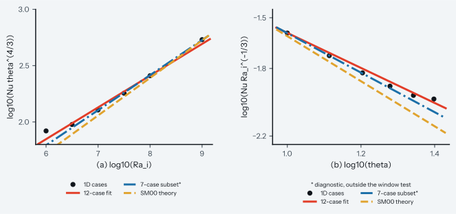
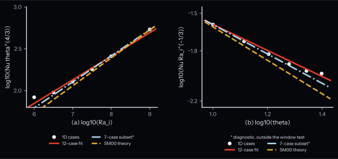
Figure: Steady-state internal-heating Nusselt number scalings against internal Rayleigh number (panel a) and Frank-Kamenetskii viscosity-contrast parameter (panel b).
How to read the plot. Panel (a) plots \(\log_{10}(\mathrm{Nu}\,\theta^{4/3})\) against \(\log_{10}(\mathrm{Ra}_i)\) at design \(\theta = 15\). Panel (b) plots \(\log_{10}(\mathrm{Nu}\,\mathrm{Ra}_i^{-1/3})\) against \(\log_{10}(\theta)\) at design \(\mathrm{Ra}_i = 10^7\). Circles show the 12 steady-state 1-D runs. The solid line is the 12-case ordinary least-squares fit, and the dash-dotted line is the 7-case convecting fit. The dashed line is the Solomatov and Moresi (2000)8 asymptotic slope (\(\beta = 1/3\) in panel a, \(-\alpha = -4/3\) in panel b). Low-\(\mathrm{Ra}_i\) and high-\(\theta\) points flatten onto the conduction floor.
Known limit. Both the 12-case design-parameter fit (\(\beta = 0.2819 \pm 0.0134\), \(\alpha = 1.0366 \pm 0.0971\)) and the realized-state fit (\(\beta_\text{real} = 0.1128 \pm 0.0286\), \(\alpha_\text{real} = -0.0786 \pm 0.4398\)) fall below the Newtonian (\(n = 1\)) acceptance window \(\beta \in [0.294, 0.350]\) and \(\alpha \in [1.294, 1.350]\) of Solomatov and Moresi (2000)8. This is consistent with low-vigor cases that cool onto the discrete pure-conduction floor and with the exponential top slope that levels off at high viscosity contrast. The test pins the current steady-state values and regressions to \(10^{-7}\) relative.
Test details
- Reference: Newtonian (\(n = 1\)) internal-heating stagnant-lid scaling theory and numerical fits of Solomatov and Moresi (2000)8, pp. 21797-21798, sec. 3; p. 21800, Table 4 and eqs. 9, 10, 12; p. 21801, Table 5; p. 21803, Table 6 rows 6-8; p. 21805, sec. 7.4, Korenaga (2009)5, p. 156, eq. 20; p. 157, Table 1; p. 158, eqs. 29-30, and Reese et al. (2005)7, p. 366, Table 2 and eq. 20.
- Tolerance: Pinned to
1e-07relative for deterministic single-process evaluation (both the 12-case design-value fit \(\beta = 0.2819 \pm 0.0134\), \(\alpha = 1.0366 \pm 0.0971\) and the realized-state fit \(\beta_\text{real} = 0.1128 \pm 0.0286\), \(\alpha_\text{real} = -0.0786 \pm 0.4398\) fall below the acceptance window \(\beta \in [0.294, 0.350]\) and \(\alpha \in [1.294, 1.350]\)). - Test id:
tests/test_mlt_calibration_smoke.py::test_stagnant_lid_scaling_exponents - Command:
pytest tests/test_mlt_calibration_smoke.py -k test_stagnant_lid_scaling_exponents(add--validation-plotsto write the plot pair; regenerate the benchmark file withpython tools/verification/generate_ssc_scaling_exponents_benchmarks.py --full)
-
M. Armann, P. J. Tackley, Simulating the thermochemical magmatic and tectonic evolution of Venus's mantle and lithosphere: Two-dimensional models, Journal of Geophysical Research: Planets, 117, E12003, 2012. SciX. ↩
-
F. Deschamps, K. Vilella, Scaling Laws for Mixed-Heated Stagnant-Lid Convection and Application to Europa, Journal of Geophysical Research: Planets, 126, e2021JE006963, 2021. SciX. ↩↩↩↩
-
B. J. Foley, D. Bercovici, Scaling laws for convection with temperature-dependent viscosity and grain-damage, Geophysical Journal International, 199, 580–603, 2014. SciX. ↩↩
-
S.-I. Karato, P. Wu, Rheology of the Upper Mantle: A Synthesis, Science, 260, 771–778, 1993. SciX. ↩
-
J. Korenaga, Scaling of stagnant-lid convection with Arrhenius rheology and the effects of mantle melting, Geophysical Journal International, 179, 154–170, 2009. SciX. ↩↩↩↩↩↩↩↩↩↩↩↩↩↩↩↩
-
L. Moresi, V. Solomatov, Mantle convection with a brittle lithosphere: thoughts on the global tectonic styles of the Earth and Venus, Geophysical Journal International, 133, 669–682, 1998. SciX. ↩↩
-
C. C. Reese, V. S. Solomatov, J. R. Baumgardner, Scaling laws for time-dependent stagnant lid convection in a spherical shell, Physics of the Earth and Planetary Interiors, 149, 361–370, 2005. SciX. ↩↩
-
V. S. Solomatov, L.-N. Moresi, Scaling of time-dependent stagnant lid convection: Application to small-scale convection on Earth and other terrestrial planets, Journal of Geophysical Research, 105, 21795–21817, 2000. SciX. ↩↩↩↩↩↩↩↩↩↩
-
P. J. Tackley, M. Ammann, J. P. Brodholt, D. P. Dobson, D. Valencia, Mantle dynamics in super-Earths: Post-perovskite rheology and self-regulation of viscosity, Icarus, 225, 50–61, 2013. SciX. ↩↩