Solid-state convection and stagnant-lid rheology
This tutorial walks through running Aragog with temperature-, pressure-, and stress-dependent solid-state mantle rheology ([phase_solid.rheology]). Starting from the bundled abe_solid.toml template, we compare a constant-viscosity solid mantle (enabled = false) against an Arrhenius diffusion-creep mantle (enabled = true), inspect the stagnant-lid boundary-layer diagnostics on solver.state.lid_state, and lower the Byerlee yield stress to observe plastic yielding in the cold upper boundary layer.
For the mathematical formulation and benchmark comparisons, see Solid-state convection and Configuration: phase_solid.rheology.
Prerequisites
- Aragog is installed (
pip install -e .). - The SPIDER-format pressure-entropy EOS tables are staged on disk (see First-run tutorial for the
spider_eos_test_data.tar.gzdownload commands andARAGOG_TEST_EOS_DIR).
1. Enable [phase_solid.rheology] in a TOML configuration
Scaffold a working configuration from the bundled abe_solid template:
aragog new ssc_demo --from abe_solid
To turn on solid-state rheology in ssc_demo.toml, set viscosity = 3.0e+17 in the existing [phase_solid] section and append a [phase_solid.rheology] table:
[phase_solid.rheology]
enabled = true
stress_closure_mode = "lid"
g_homologous = 25.0
t_sol_0 = 1400.0
arrhenius_t_ref = 1600.0
viscosity_max_log10 = 40.0
yield_stress_c = 50.0e6
yield_stress_mu = 0.6
yield_stress_max = 500.0e6
s_top_inf = 0.22
c_theta = 0.15
When enabled = false (the default), [phase_solid].viscosity is a uniform solid-phase dynamic viscosity (\(\eta_\mathrm{solid} = 3.0e+17\,\mathrm{Pa\,s}\)). When enabled = true, [phase_solid].viscosity is the reference viscosity \(\eta_0\) at \((T_\mathrm{ref}, P = 0)\) on the reference solidus t_sol_0, and the solver evaluates the two-pass stagnant-lid closure (stress_closure_mode = "lid", the default mode when enabled) at every right-hand-side call.
2. Compare rheology-off and rheology-on runs from Python
The script below loads cfg/abe_solid.toml (or ssc_demo.toml via Parameters.from_file), sets an initial entropy profile \(S(r) = 2050.0 - 1720.0\,(0.2\,\xi + 0.8\,\xi^4)\,\mathrm{J/(kg\,K)}\) spanning from \(2050.0\,\mathrm{J/(kg\,K)}\) at the core-mantle boundary to \(330.0\,\mathrm{J/(kg\,K)}\) at the surface, integrates for \(10.0\,\mathrm{yr}\), and prints every comparison quantity for enabled = False (default) and enabled = True:
from dataclasses import replace
import importlib.resources
import os
from pathlib import Path
import numpy as np

from aragog.eos import EntropyEOS
from aragog.parser import Parameters
from aragog.rheology import SolidRheologyParams
from aragog.solver import EntropySolver

eos_dir = Path(os.environ["ARAGOG_TEST_EOS_DIR"])
cfg_path = Path(str(importlib.resources.files("aragog").joinpath("cfg/abe_solid.toml")))


def run_case(rheology: SolidRheologyParams) -> EntropySolver:
    params = Parameters.from_file(cfg_path)
    params.boundary_conditions = replace(
        params.boundary_conditions,
        core_bc="quasi_steady",
        inner_boundary_condition=1,
    )
    params.solver.end_time = 10.0
    params.energy.kappah_floor = 0.0
    params.phase_solid = replace(
        params.phase_solid,
        viscosity=3.0e+17,
        rheology=rheology,
    )
    solver = EntropySolver(params, EntropyEOS(eos_dir))
    solver.initialize()
    n_stag = params.mesh.number_of_nodes - 1
    xi = np.linspace(0.0, 1.0, n_stag)
    s_init = 2050.0 - 1720.0 * (0.2 * xi + 0.8 * xi**4)
    solver.set_initial_entropy(s_init)
    solver.solve()
    out = solver.get_state()
    solver.dSdt(params.solver.end_time, out.S_final)
    return solver


solver_off = run_case(SolidRheologyParams(enabled=False))
solver_on = run_case(SolidRheologyParams(enabled=True))

for label, solver in (("off", solver_off), ("on", solver_on)):
    out = solver.get_state()
    visc_b = np.asarray(solver.state.phase_basic.viscosity()).ravel()
    eta_diff_b = np.asarray(solver.state.phase_basic.eta_diff()).ravel()
    print(
        f"Rheology {label}: status={out.status}, "
        f"eta_surf={visc_b[-1]:.3e} Pa s, "
        f"eta_cmb={visc_b[0]:.3e} Pa s, "
        f"eta_diff_cmb={eta_diff_b[0]:.3e} Pa s, "
        f"max_jconv={np.max(out.jconv_b):.2f} W/m^2, "
        f"max_kappah={np.max(out.eddy_diff):.4f} m^2/s, "
        f"T_magma={out.T_magma:.2f} K, "
        f"T_core={out.T_core:.2f} K"
    )
With the CI test EOS tables, the two runs produce:
| Quantity | enabled = False (default) |
enabled = True (stress_closure_mode = "lid") |
|---|---|---|
Solver status (out.status) |
0 |
0 |
Surface viscosity \(\eta_\mathrm{surf}\) (phase_basic.viscosity()[-1]) [Pa s] |
$3.000e+17$ |
$9.076e+27$ |
Bulk CMB viscosity \(\eta_\mathrm{cmb}\) (phase_basic.viscosity()[0]) [Pa s] |
$1.664e+17$ |
$1.916e+18$ |
Solid CMB diffusion viscosity \(\eta_\mathrm{diff,cmb}\) (phase_basic.eta_diff()[0]) [Pa s] |
$3.000e+17$ |
$3.601e+18$ |
Peak convective heat flux \(\max(F_\mathrm{conv})\) (np.max(out.jconv_b)) [W/m\(^2\)] |
$161063.04$ |
$534.83$ |
Peak eddy diffusivity \(\max(\kappa_h)\) (np.max(out.eddy_diff)) [m\(^2\)/s] |
$15.6253$ |
$0.0573$ |
Near-surface magma temperature \(T_\mathrm{magma}\) (out.T_magma) [K] |
$782.15$ |
$782.06$ |
Core temperature \(T_\mathrm{core}\) (out.T_core) [K] |
$3566.07$ |
$3566.07$ |
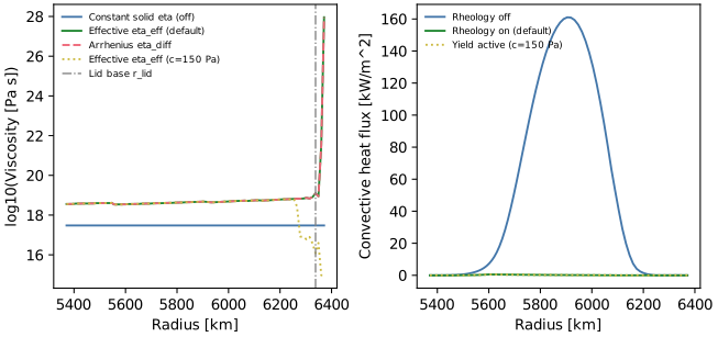
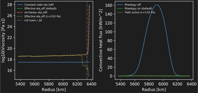
With enabled = False, the cold upper boundary layer keeps the uniform solid viscosity (\(\eta_\mathrm{surf} = 3.000e+17\,\mathrm{Pa\,s}\)), and the convective heat flux peaks at \(\max(F_\mathrm{conv}) = 161063.04\,\mathrm{W/m^2}\), about 470 km below the surface. With enabled = True, Arrhenius stiffening raises the surface viscosity to \(\eta_\mathrm{surf} = 9.076e+27\,\mathrm{Pa\,s}\) and forms a conductive stagnant lid: above its base the convective heat flux is below 0.01 W/m\(^2\), and the peak falls to \(\max(F_\mathrm{conv}) = 534.83\,\mathrm{W/m^2}\), about 770 km below the surface (see the profile figure). At the partially molten CMB node, phase_basic.eta_diff()[0] reports the pure solid-phase diffusion viscosity (\(3.000e+17\,\mathrm{Pa\,s}\) vs \(3.601e+18\,\mathrm{Pa\,s}\)), whereas phase_basic.viscosity()[0] blends that solid viscosity with the liquid phase across the melt fraction (\(1.664e+17\,\mathrm{Pa\,s}\) vs \(1.916e+18\,\mathrm{Pa\,s}\)).
The start profile follows the node index: xi = np.linspace(0.0, 1.0, n_stag) spaces \(\xi\) evenly over the staggered nodes, not over the radius. The node radii depend on the mesh (this run has a 3000 m cell at the core-mantle boundary and mass coordinates), so the same script sets a different profile in radius on each mesh, and the rheology-on peak changes with it:
| Start profile | Mesh | Peak \(F_\mathrm{conv}\) [W/m\(^2\)] |
|---|---|---|
| even in node index | this mesh, 100 nodes | 534.83 |
| even in node index | this mesh, 400 nodes | 167.27 |
| even in radius, \(\xi = (r - r_0)/(r_{N-1} - r_0)\) | this mesh, 100 nodes | 215.21 |
| even in radius | uniform mesh, 100 nodes | 219.47 |
| even in radius | this mesh, 400 nodes | 147.69 |
In the rows even in radius, \(r\) is the radius of each staggered node, and \(r_0\) and \(r_{N-1}\) are the radii of the first and the last of the \(N\) staggered nodes.
The peak is not converged at 100 nodes; the run of this page compares enabled = False with enabled = True on one mesh.
3. Read the stagnant-lid diagnostics
When enabled = True and stress_closure_mode = "lid", solver.state.lid_state stores the boundary-layer diagnostics computed by compute_stagnant_lid_state at the most recent state evaluation:
lid = solver_on.state.lid_state
print(f"has_lid:     {lid['has_lid']}")
print(f"d_lid:       {float(lid['d_lid']) * 1e-3:.2f} km")
print(f"r_lid_base:  {float(lid['r_lid_base']) * 1e-3:.2f} km")
print(f"T_i:         {float(lid['T_i']):.2f} K")
print(f"T_lid:       {float(lid['T_lid']):.2f} K")
print(f"theta:       {float(lid['theta']):.3f}")
print(f"dT_rh:       {float(lid['dT_rh']):.2f} K")
print(f"eta_i:       {float(lid['eta_i']):.3e} Pa s")
print(f"tau_d_lid:   {float(lid['tau_d_lid']) * 1e-3:.2f} kPa")
print(f"tau_y_lid:   {float(lid['tau_y_lid']) * 1e-6:.2f} MPa")
print(f"w_y:         {float(lid['w_y']):.3e}")
For the enabled = True run at \(t = 10.0\,\mathrm{yr}\), these diagnostics evaluate to:
has_lid = True, with conductive lid thickness \(d_\mathrm{lid} = 33.11\,\mathrm{km}\) (\(d_\mathrm{lid} = 33106.60\,\mathrm{m}\)) and lid-base radius \(r_\mathrm{lid,base} = 6337.89\,\mathrm{km}\).- Convecting interior temperature \(T_i = 2012.48\,\mathrm{K}\), lid temperature \(T_\mathrm{lid} = 1449.30\,\mathrm{K}\), and lid-base isotherm target \(T_\mathrm{lid,iso} = 1834.80\,\mathrm{K}\).
- Frank-Kamenetskii parameter \(\theta = 15.235\), rheological temperature scale \(\Delta T_\mathrm{rh} = 80.76\,\mathrm{K}\), and interior viscosity \(\eta_i = 5.161e+18\,\mathrm{Pa\,s}\).
- Lid-scaled convective driving stress \(\tau_{d,\mathrm{lid}} = 831.52\,\mathrm{kPa}\) (\(831522.45\,\mathrm{Pa}\)) against a Byerlee lid yield strength of \(\tau_{y,\mathrm{lid}} = 500.00\,\mathrm{MPa}\), so the plastic yielding weight is \(w_y = 2.131e-09\) (
0yielding basic nodes) and the lid remains in the unyielded stagnant-lid regime.
4. Modify yield parameters to trigger plastic lid mobilisation
To observe plastic yielding in Pass 2 of the stress closure, lower the cohesion yield_stress_c below \(\tau_{d,\mathrm{lid}} = 831.52\,\mathrm{kPa}\) and set yield_stress_mu = 0.0:
solver_yield = run_case(
    SolidRheologyParams(
        enabled=True,
        stress_closure_mode="lid",
        yield_stress_c=150.0,
        yield_stress_mu=0.0,
        yield_stress_max=1.0e8,
    )
)
lid_yield = solver_yield.state.lid_state
eta_diff = np.asarray(solver_yield.state.phase_basic.eta_diff()).ravel()
eta_eff = solver_yield.state.eta_eff_basic
n_yielding = int(np.sum(eta_eff < eta_diff * (1.0 - 1.0e-12)))
print(f"w_y = {float(lid_yield['w_y']):.1f}, yielding nodes = {n_yielding}")
print(f"Surface eta_diff = {eta_diff[-1]:.3e} Pa s -> eta_eff = {eta_eff[-1]:.3e} Pa s")
With yield_stress_c = 150.0 Pa and yield_stress_mu = 0.0:
- The lid yield strength is \(\tau_{y,\mathrm{lid}} = 150.0\,\mathrm{Pa}\), below \(\tau_{d,\mathrm{lid}} = 831.16\,\mathrm{kPa}\).
- The yielding blend weight reaches \(w_y = 1.0\), and
13basic nodes inside the upper boundary layer yield plastically (eta_eff < eta_diff). - At the surface basic node, plastic yielding reduces the effective viscosity from \(\eta_\mathrm{diff,surf} = 8.919e+27\,\mathrm{Pa\,s}\) to \(\eta_\mathrm{eff,surf} = 9.315e+14\,\mathrm{Pa\,s}\). The lid then carries convective heat flux near the surface: about 11 km down it rises from below 0.01 to about 64 W/m\(^2\). The peak deep in the mantle changes by less than 0.1 % (534.83 to 534.87 W/m\(^2\)).