Phase transitions
What this page checks
This page checks how Aragog changes the material properties of the mantle (heat capacity, density, expansivity, adiabatic gradient and viscosity) when the entropy of a node crosses the solidus or the liquidus (see Phase transitions), and where the expansivity of a single phase comes from (see thermal expansivity of a single phase). Validation here means that we run the phase evaluator on the SPIDER test tables, where the right answer follows from the blend formula, and check that Aragog gives that answer. If this part were wrong, the heat flux through a cell face would jump when a node starts or stops to melt, and the solver would take very small time steps there. Each case below says why the check exists, what it tests, how we know the right answer and why it matters, then shows a plot or says why it has none, and the test details.
All cases use the SPIDER P-S test tables (ARAGOG_TEST_EOS_DIR, Build tests) on a mesh from the core-mantle boundary (146 GPa) to the surface (0 GPa): 12 nodes in the first three cases and 10 nodes in the JAX case. The last three cases check the source of the expansivity outside and on the edges of the mushy zone, at the same 12 pressures (the mush case at 12 pressures from 0 to 145 GPa). The symbol \(g = (S - S_\mathrm{sol}) / (S_\mathrm{liq} - S_\mathrm{sol})\) is the melt coordinate: 0 on the solidus, 1 on the liquidus, below 0 in the solid and above 1 in the liquid. The width \(w\) is the setting matprop_smooth_width; the default is 0.01.
On each boundary, a property is the mean of its two values
Why this check exists. Near a boundary every property has two values: the two-phase value of the mushy zone and the single-phase value from the solid or the melt table. If the code gave the wrong weight on the boundary, for example 1 as with \(w = 0\), the property would take the two-phase value alone. On the test tables the two values of the heat capacity differ by 3.5 % to a factor of 23, so the test sees that error at every pressure.
What it tests. The test puts every node exactly on the solidus (\(g = 0\)), then exactly on the liquidus (\(g = 1\)), at the default width. It compares the heat capacity, the density, the adiabatic gradient \((\partial T/\partial P)_S\) and the logarithm of the viscosity with the mean of the two values. It takes the two-phase value from the evaluator at \(w = 0\), which uses weight 1 on the boundary, and the single-phase value from the tables directly. The two values of the density are the same on the boundary, so the density is compared but does not test the weight; the test asserts the gap between the two values for the heat capacity.
How we know the right answer. SPIDER's get_smoothing (util.c) gives the two-phase value the weight \(\tfrac{1}{2}[1 + \tanh(g/w)]\) below \(g = 0.5\) and \(\tfrac{1}{2}[1 - \tanh((g - 1)/w)]\) above it. Both are exactly \(\tfrac{1}{2}\) on the boundary for any \(w > 0\), so each property is the mean of its two values. The expansivity is not compared, because the evaluator changes negative values after the blend with a function that is not linear.
Why it matters. The properties on the boundary set the heat flux of a node that is just starting to melt or to freeze.
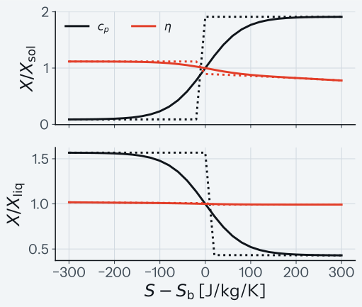
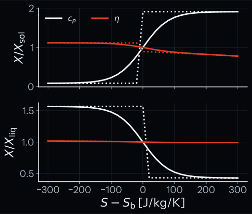
How to read the plot. Top: the solidus; bottom: the liquidus, both at 65.7 GPa. The horizontal axis is the entropy minus the entropy of the boundary, in J/kg/K. The vertical axis is a property \(X\) divided by its value on the boundary. Solid lines use the default width 0.01, dotted lines width 0. Solid lines pass through 1 on the boundary and change smoothly over about 81 J/kg/K (0.01 of the melting interval of 8148 J/kg/K). Dotted lines jump there; the jump looks like a steep line only because the points are 20 J/kg/K apart.
Test details
- Reference: SPIDER
get_smoothing(util.c): the weight is \(\tfrac{1}{2}\) at \(g = 0\) and \(g = 1\) for any \(w > 0\). - Tolerance: 10⁻¹² relative at all 12 node pressures, for the heat capacity, the density, the adiabatic gradient and the logarithm of the viscosity (measured: 0).
- Discrimination: the two values of the heat capacity differ by at least 155 % of the mean at the solidus and 3.5 % at the liquidus; the test asserts more than 2 %, so a weight of 0 or 1 on the boundary fails.
- Test id:
tests/test_matprop_smooth_width_validation.py::test_on_each_boundary_every_property_is_the_mean_of_the_two_branches - Command:
pytest tests/test_matprop_smooth_width_validation.py -k mean(add--validation-plotsto write the plot pair)
No jump at the solidus and the liquidus
Why this check exists. With \(w = 0\), or with a weight that jumps, a property changes by a finite step between two entropies that are almost equal. On the test tables the heat capacity then jumps by a factor of 7.9 to 23 at the solidus.
What it tests. The test puts every node 10⁻⁹ J/kg/K below a boundary, then 10⁻⁹ J/kg/K above it, at the default width. It compares the heat capacity, the density, the expansivity, the adiabatic gradient and the logarithm of the viscosity between the two states.
How we know the right answer. The weight changes by about \(10^{-9} / (w \Delta S)\) over that step, with \(\Delta S = S_\mathrm{liq} - S_\mathrm{sol}\) between 2563 and 8394 J/kg/K on this mesh. A continuous property therefore changes by far less than 10⁻⁶ of its value.
Why it matters. A step in a property gives a step in the heat flux through a face, and the time stepper must then take very small steps each time a node crosses a boundary.
This case has no plot of its own: the plot of the case above shows the same curves near both boundaries.
Test details
- Reference: continuity of the blend for \(w > 0\).
- Tolerance: 10⁻⁶ relative at all 12 node pressures (measured: at most 1.2 × 10⁻⁷, at the surface node, where the blended expansivity is negative, −2.1 × 10⁻⁴ 1/K, and the clamp of negative values maps it to 1.2 × 10⁻¹³ 1/K, so a round-off change of the blended value shows as a larger relative change; below 3 × 10⁻¹¹ at the other nodes).
- Discrimination: at \(w = 0\) the heat capacity jumps by more than a factor of 7 at every node at the solidus (measured 7.9 to 23).
- Test id:
tests/test_matprop_smooth_width_validation.py::test_the_default_width_keeps_every_property_continuous_across_the_boundary - Command:
pytest tests/test_matprop_smooth_width_validation.py -k continuous
Far from both boundaries the width changes nothing
Why this check exists. The blend must only act near the boundaries. If the width leaked into the solid, the deep mushy zone or the liquid, a change of the width would change runs that never come near a boundary.
What it tests. The test puts every cell at \(g = -0.25\), \(0.35\) and \(1.3\), and checks first that every node, the surface node included, is at least 0.2 in \(g\) from both boundaries. It then compares the right-hand side of the entropy equation at the default width and at \(w = 0\). As a control, it repeats this with every cell at \(g = 0.02\), inside the blend.
How we know the right answer. More than 0.2 from a boundary, \(|g/w|\) or \(|(g - 1)/w|\) is at least 20, and \(\tanh(20)\) rounds to exactly 1 in double precision. The weight is then exactly 0 or 1, as at \(w = 0\).
Why it matters. It shows that the default only changes states near a phase boundary.
This case has no plot: it checks that two arrays are equal bit for bit.
Test details
- Reference: \(\tanh(20) = 1\) in double precision.
- Tolerance: bit-identical right-hand side in all 3 states; at \(g = 0.02\) the right-hand sides differ.
- Test id:
tests/test_matprop_smooth_width_validation.py::test_far_from_both_boundaries_the_rhs_does_not_change_with_the_width - Command:
pytest tests/test_matprop_smooth_width_validation.py -k far_from
The JAX right-hand side follows the width
Why this check exists. The production solver uses the JAX right-hand side and its Jacobian. If the JAX kernel blended the properties with a different width from the NumPy evaluator, the two would disagree near every boundary.
What it tests. The test puts 9 cells at \(g\) = −0.02, −0.005, 0, 0.004, 0.012, 0.5, 0.99, 1 and 1.015, on both sides of both boundaries. A test helper builds the JAX parameters with the width of the configuration, as PROTEUS does in a coupled run; Aragog itself does not build JAX parameters from a configuration. The test compares the JAX right-hand side with the NumPy one at the default width. As a control, it sets the JAX width to 0. This case does not test the weight exactly on a boundary: with that weight set to 1 in the NumPy evaluator it still passes, and the first case fails.
How we know the right answer. The NumPy evaluator is the reference; both paths use the same blend formula.
Why it matters. A difference between the two paths would make the Jacobian of the solver wrong near a boundary.
This case has no plot: it checks the agreement of two arrays to round-off.
Test details
- Reference: the NumPy right-hand side.
- Tolerance: 10⁻¹⁰ relative (measured: 5.9 × 10⁻¹⁵); at JAX width 0 the difference is more than 10⁻⁶ (measured: a relative difference of 6.1).
- Test id:
tests/test_matprop_smooth_width_validation.py::test_the_jax_rhs_matches_numpy_inside_the_blend_at_the_default_width - Command:
pytest tests/test_matprop_smooth_width_validation.py -k jax_rhs
NumPy and JAX take the same single-phase expansivity
Why this check exists. Outside the mushy zone the expansivity comes from the identity \(\alpha = \rho\, c_p\, (\partial T/\partial P)_S / T\) in both the NumPy evaluator and the JAX right-hand side (thermal expansivity of a single phase). Many table directories, the SPIDER test tables among them, also carry thermal_exp files. If the NumPy path read those files, a NumPy run and a JAX run of the same case would integrate different expansivities: on the test tables they differ from the identity by \(7.6 \times 10^{-7}\) to \(7.9 \times 10^{-4}\) relative at the states of this case.
What it tests. The test puts the mantle at 72 states: 50, 200 and 500 J/kg/K below the solidus and above the liquidus, at the 12 node pressures from 0 to 146 GPa, all inside the tables. It compares the expansivity of the NumPy evaluator with that of the JAX evaluate_phase, at width 0.01 (where the two-phase weight reaches 0.23 at 50 J/kg/K from a boundary) and at width \(10^{-6}\) (where the weight is 0). At width \(10^{-6}\) it also compares the NumPy expansivity with the identity of the evaluator's own density, heat capacity, adiabatic gradient and temperature. A second test compares EntropyEOS.thermal_expansivity and material_expansivity with the JAX methods at the same states.
How we know the right answer. The identity follows from the Maxwell relation \((\partial T/\partial P)_S = (\partial V/\partial S)_P\), and the JAX path is a second implementation of it. Agreement to round-off shows that both paths take \(\alpha\) from the same source.
Why it matters. With a JAX factory, CVODE integrates the JAX right-hand side and Aragog reports the heat flux of the NumPy one; the two agree only when both use the same expansivity. This holds under the default cp_blend = "latent": the JAX path has no linear branch.
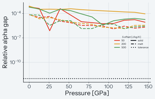
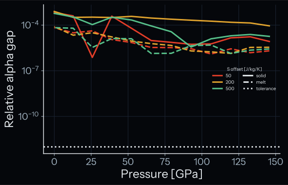
How to read the plot. The horizontal axis is the pressure. The vertical axis is the relative difference between the expansivity of the thermal_exp tables and the identity, on a log scale. The colour gives the entropy offset from the boundary in J/kg/K, solid lines the solid states and dashed lines the melt states. The plot shows the error that the NumPy path would have if it read these tables; the solver does not read them, so this gap does not enter a run. The dotted line is the tolerance of the NumPy and JAX agreement, \(10^{-12}\); the measured agreement lies below it at every state.
Test details
- Reference: the identity \(\alpha = \rho\, c_p\, (\partial T/\partial P)_S / T\) and the JAX implementation of it.
- Tolerance: 10⁻¹² relative at all 72 states (measured: 4.3 × 10⁻¹⁵ at width 0.01, 6.5 × 10⁻¹⁶ at width 10⁻⁶, 6.9 × 10⁻¹⁶ for both
EntropyEOSmethods). - Discrimination: with the NumPy expansivity from the
thermal_exptables all 4 comparisons fail, by up to 8.0 × 10⁻⁴. The plot test pins the gap range of the plot, 7.56 × 10⁻⁷ to 7.87 × 10⁻⁴, to 1 %. - Sign convention: on a table copy with a negative solid gradient, the evaluator clamps \(\alpha\) to about 0 and the
EntropyEOSmethods give \(|\alpha|\) (the test tables hold no negative gradient). - PR tier: one unit test checks the NumPy and JAX agreement at a solid and a melt state at 50 GPa.
- Test ids:
tests/test_alpha_identity_validation.py::test_numpy_and_jax_single_phase_alpha_agree_on_tables_with_thermal_exp,::test_numpy_and_jax_eos_expansivity_methods_agree_on_tables_with_thermal_exp,::test_the_thermal_exp_table_alpha_differs_from_the_identity(the plot),::test_numpy_and_jax_alpha_agree_in_the_cold_solid_at_the_surface,::test_the_composite_blend_takes_the_identity_alpha_outside_the_mush,::test_the_sign_conventions_of_the_identity_on_a_negative_gradient,::test_numpy_and_jax_alpha_agree_at_one_solid_and_one_melt_state - Command:
pytest tests/test_alpha_identity_validation.py(add--validation-plotsto write the plot pair)
The mushy-zone expansivity keeps its two-phase value
Why this check exists. Under the default cp_blend = "latent" the two-phase expansivity of the mushy zone is the composite formula of SPIDER, the same in NumPy and JAX. The source of the single-phase expansivity must not change that value; it enters the blended expansivity only through the weight \(1 - \mathrm{smth}\), which is close to \(\tfrac{1}{2}\) within about one width of each boundary and close to 0 deeper in the mushy zone.
What it tests. The test reads 60 states at melt fractions 0.002, 0.1, 0.5, 0.9 and 0.998 at 12 pressures from 0 to 145 GPa, with their expansivity at width 0 and 0.01 as tools/verification/generate_alpha_mush_reference.py writes it on these tables with the single-phase expansivity read from the thermal_exp tables (tests/validation/data/alpha_mush_2d1af473.csv). Its header names the code version and the table checksums, and the test checks both against the tables in use. At width 0 the expansivity is the two-phase value alone and must be equal to rounding, 10⁻¹⁴ relative (Linux and macOS differ by up to 2 units in the last place). At width 0.01 the single-phase value enters with the weight \(1 - \mathrm{smth}\), so the expansivity may change by at most that weight times the gap between the table and the identity value, plus 10⁻¹³ relative. At melt fractions 0.002 and 0.998, where the weight is 0.40, the change must equal that product to 10⁻⁶ relative wherever the clamp is inactive. The test also compares the NumPy and the JAX expansivity at all 60 states, at widths 0 and 0.01.
How we know the right answer. The blend is linear in the single-phase value, and the clamp of negative values after it does not increase a difference.
Why it matters. A cooling magma ocean passes through the mushy zone, where this expansivity sets the buoyancy of the convective flux.
This case has no plot: it checks equality and a bound on 60 numbers.
Test details
- Reference: the stored expansivity of the same states, with the single-phase value from the
thermal_exptables; the two-phase formula is the same. - Tolerance: 10⁻¹⁴ relative at width 0 (10⁻²⁰ 1/K absolute for the 5 states at 0 GPa that the clamp holds at 5.1 × 10⁻¹⁴ to 6.1 × 10⁻¹⁴ 1/K); at width 0.01 the bound above, with equality at the 0.002 and 0.998 states above \(10^{-8}\) 1/K; NumPy against JAX to 10⁻¹² relative.
- Measured, width 0.01 against the stored values: 46 of 60 states change; the largest change is 3.3 × 10⁻⁹ 1/K, 1.0 × 10⁻⁵ relative, at melt fraction 0.998 and 13.2 GPa; the largest relative change is 6.2 × 10⁻⁵ at 0 GPa, where the clamp holds the expansivity near 2 × 10⁻¹³ 1/K.
- Measured, NumPy against JAX at the 60 states: 9.3 × 10⁻¹⁶ at width 0 and 9.0 × 10⁻¹⁶ at width 0.01.
- Test id:
tests/test_alpha_identity_validation.py::test_the_mush_alpha_changes_only_through_the_single_phase_weight - Command:
pytest tests/test_alpha_identity_validation.py -k mush
The linear blend meets the single-phase expansivity on each boundary
Why this check exists. Under cp_blend = "linear" the two-phase expansivity interpolates between the values of the two phases on the solidus and the liquidus. If those values came from a different source than the single-phase expansivity, \(\alpha\) would step on each boundary.
What it tests. The test puts every node exactly on the solidus, then exactly on the liquidus, at width 0 under cp_blend = "linear", at the 12 node pressures. It compares the expansivity with the identity value of that phase from the tables, after the clamp. At melt fraction 0.3 it compares the expansivity with \(0.3\) times the liquidus value plus \(0.7\) times the solidus value.
How we know the right answer. At melt fraction 0 or 1 the linear blend is the value of one phase, and both come from the identity.
Why it matters. A step in \(\alpha\) gives a step in the convective heat flux when a node crosses a boundary.
This case has no plot: it checks the agreement of two arrays to round-off.
Test details
- Reference: the identity of each phase on the boundary.
- Tolerance: 10⁻¹² relative (measured: 0 at both boundaries).
- Test id:
tests/test_alpha_identity_validation.py::test_the_linear_blend_meets_the_single_phase_alpha_at_each_boundary - Command:
pytest tests/test_alpha_identity_validation.py -k linear