First-principles verification
What this page checks
This page checks the numerical solvers and physical conservation laws in Aragog. Aragog solves the coupled equations of energy conservation, hydrostatic pressure, and mantle convection to simulate magma-ocean cooling and solid-mantle thermal evolution. Validation here means running the solver on cases where another source provides the known answer. The test then checks that the code matches that answer inside a stated numerical tolerance. Known answers come from analytical limits, physical conservation laws, published benchmark studies, or independent second code paths. If these numerical methods are wrong, the mantle calculates incorrect temperatures, melt fractions, and boundary heat fluxes. Those errors then propagate directly into atmospheric outgassing, planet contraction, and orbital evolution in PROTEUS. Each case below states why the check exists, what it tests, how we know the right answer, and why it matters. The box "Test details" at the end of each case gives the reference, the tolerance, the test id, and the test command.
Test categories
The tests are organised by the layer they cover:
EOS unit tests (tests/test_entropy_pytest.py)
Exercise EntropyEOS and EntropyPhaseEvaluator:
- Property lookups (temperature, density, heat capacity, thermal expansivity, isentropic temperature gradient) at on-grid and off-grid \((P, S)\) points.
- Solidus and liquidus entropy lookups against the reference
solidus_P-S.datandliquidus_P-S.datfiles. - Smooth-clipped melt fraction \(\phi(P, S)\): monotone in \(S\), clamped to \([0, 1]\), \(C^\infty\) through the solidus and liquidus crossings.
- The two-stage SPIDER-parity blend (cubic-Hermite or tanh smoothing followed by
combine_matprop) for density, heat capacity, and viscosity. - The latent-blend \(c_p\) method against the linear blend.
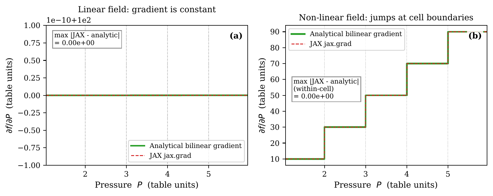
Figure 1. JAX-traced bilinear interpolation of the EOS table reproduces the numpy reference to float-64 machine precision and supplies finite, non-zero derivatives via jax.jacrev at on- and off-grid \((P, S)\) points. The agreement is the prerequisite for the analytic Jacobian path used by CVODE.
Phase evaluator tests
Test the SPIDER-parity behaviour of EntropyPhaseEvaluator:
- Phase identification at \((P, S)\) in pure solid, pure liquid, and mushy regimes.
- Viscosity tanh blend through the rheological transition \(\phi_\mathrm{rheo}\).
- Gravitational-separation velocity in viscous and inviscid regimes.
- Pressure-dependent latent heat \(L(P) = T_\mathrm{liq}(P) [S_\mathrm{liq}(P) - S_\mathrm{sol}(P)]\).
Solver integration tests
Drive EntropySolver through short integrations and check the resulting profiles:
- Standalone grey-body cooling: a fully-molten initial state cools toward the equilibrium temperature without status flag failures.
- The
set_initial_entropy,set_initial_dSdr_cmb, andset_initial_core_temperaturepaths produce the expected state-vector layouts for each of the fivecore_bcmodes. - The retry-ladder hooks (
get_current_dSdr_cmb,_atol_sf) round-trip cleanly.
Conservation tests (tests/test_entropy_verification.py)
The conservation tests are the strongest class of verification because they hold under any valid run, not just specific test scenarios:
- Energy conservation. \(E_\mathrm{th}\) change over a closed integration matches the time-integrated surface flux within solver tolerance.
- Mass conservation. Mantle mass remains constant through phase changes.
- Grey-body cooling. Surface flux follows \(\varepsilon\sigma(T_\mathrm{top}^4 - T_\mathrm{eqm}^4)\) inside tolerance once the radiative regime is established.
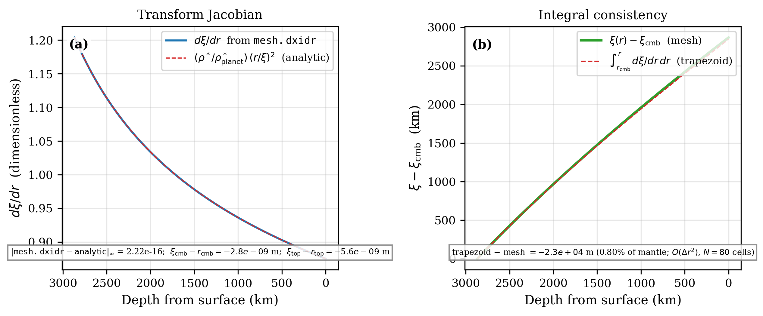
Figure 2. Mass-coordinate mesh Jacobian. The Newton solve that maps from mass coordinate to spatial radius (used when mass_coordinates = true) is monotone, smooth, and consistent with the analytic Adams-Williamson density profile. Departures here would propagate to mis-aligned cell volumes and a spurious mass-conservation residual in the integrator.
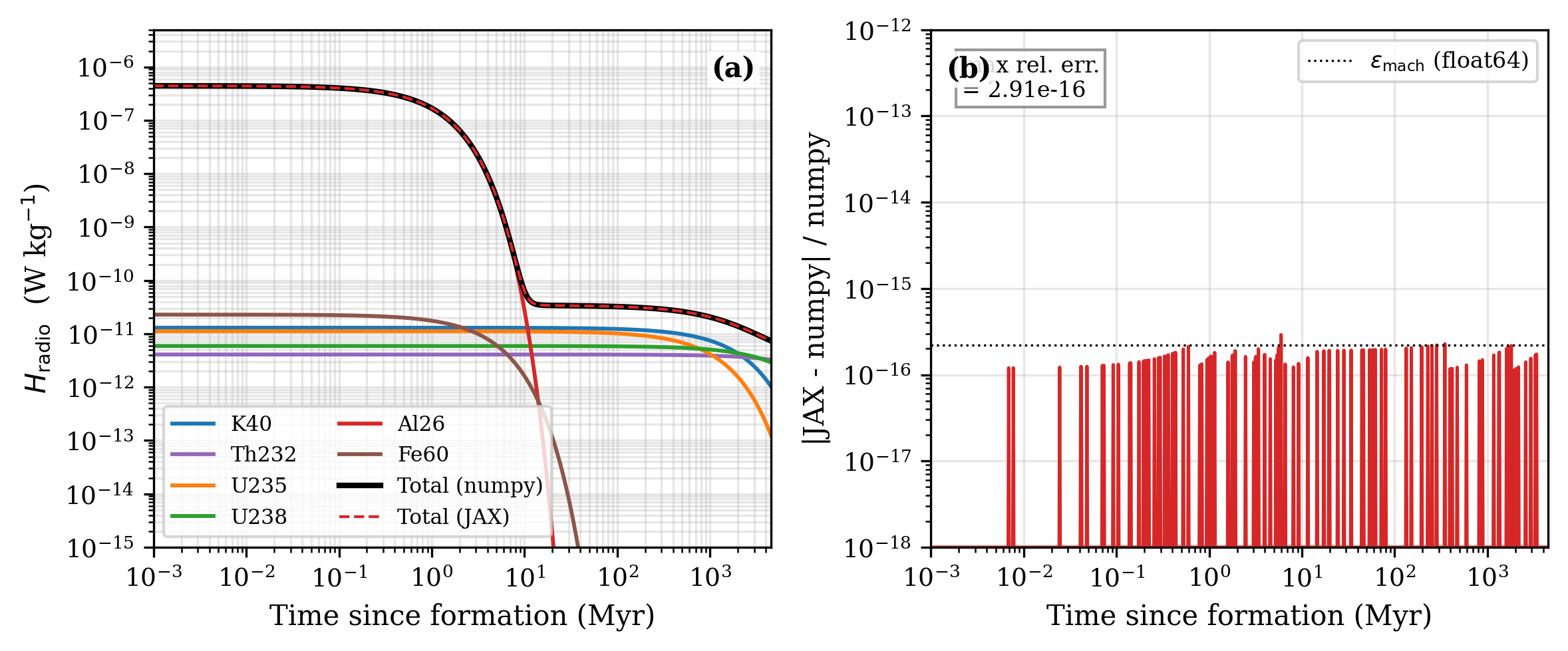
Figure 3. Radioactive heating \(H_\mathrm{radio}(t)\) per unit mass from Solar System formation to the present. (a) The 6 nuclides and their total from the NumPy and the JAX code: the long-lived \(^{40}\mathrm{K}\), \(^{232}\mathrm{Th}\), \(^{235}\mathrm{U}\) and \(^{238}\mathrm{U}\) with the present-day values of the bundled configuration (Ruedas (2017)1) decayed back to formation, and the short-lived \(^{26}\mathrm{Al}\) and \(^{60}\mathrm{Fe}\) from the initial ratios \(^{26}\mathrm{Al}/^{27}\mathrm{Al} = 5.25 \times 10^{-5}\) and \(^{60}\mathrm{Fe}/^{56}\mathrm{Fe} = 1.0 \times 10^{-8}\) in a bulk silicate Earth with 2.36 wt % Al and 6.26 wt % Fe, close to the values of Jacobsen et al. (2008)2, Tang & Dauphas (2012)3 and McDonough & Sun (1995)4. (b) Relative difference of the JAX total from the NumPy total: at most \(2.91 \times 10^{-16}\), near the float64 machine precision. Used as the source-term verification for the closed-mantle energy balance: the cumulative step_dE_Q_radio_J integral must match the time integral of \(\rho \cdot H_\mathrm{radio}\) over each call to solver tolerance.
JAX path tests (tests/test_jax_entropy.py)
Verify that the JAX-backed EntropyEOS_JAX and compute_fluxes agree with the numpy path:
- EOS parity:
EntropyEOS_JAXreturns the same temperature, density, heat capacity, thermal expansivity, \(\partial T/\partial P|_S\), and conductivity asEntropyEOSon the same \((P, S)\) inputs. - Phase evaluator parity: the JAX two-stage blend matches
EntropyPhaseEvaluatorto within floating-point tolerance. - JIT and
vmapcompatibility: the JAX flux assembly is differentiable in full withjax.grad/jax.jacrevand survives JIT compilation without recompilation hot-spots. - Boundary-copy tests:
dSdrboundary values copy from the nearest interior node (SPIDERic.c:450parity) instead of being extrapolated. - Solver parity: integrating the same problem with the JAX-RHS-driven CVODE path and the numpy RHS produces matching trajectories.
Numpy ↔ JAX RHS parity at representative magma-ocean states
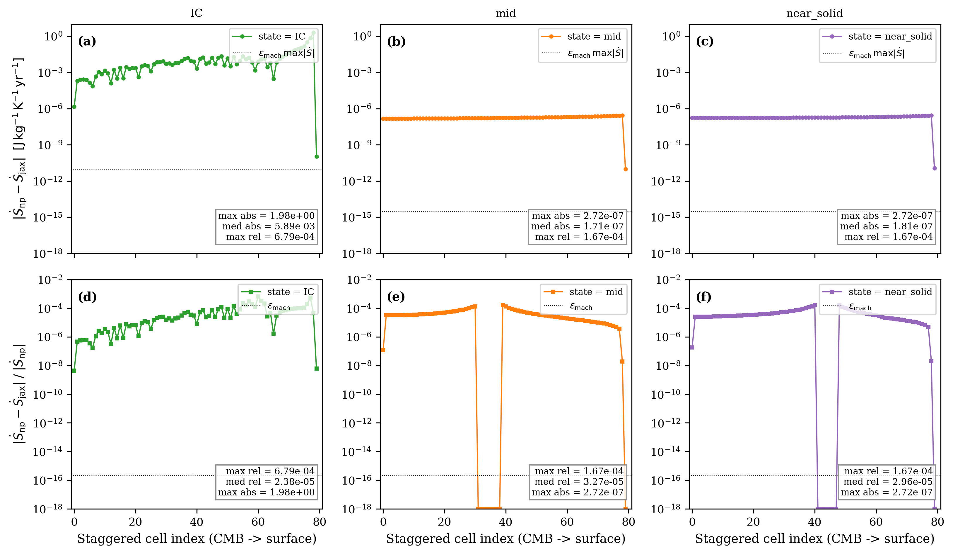
Figure 4. Numpy \(\leftrightarrow\) JAX RHS parity on an 80-cell Earth mesh at three representative magma-ocean states. Top row, panels (a-c): per-cell absolute residual \(|\dot S_\text{numpy} - \dot S_\text{jax}|\) in J/kg/K/yr; the dotted line is \(\epsilon_\mathrm{mach}\,\max|\dot S|\) (the floating-point round-off floor expected on a single FP operation). Bottom row, panels (d-f): per-cell relative residual \(|\dot S_\text{numpy} - \dot S_\text{jax}|/|\dot S_\text{numpy}|\); the dotted line is float-64 machine epsilon. The three states are (a/d) initial condition (full magma ocean, \(S \approx 3900\) J/kg/K, dimensionally uniform), (b/e) mid-solidification (\(S = 3300 \to 3700\) J/kg/K from CMB to surface), (c/f) near-solid (\(S = 3000 \to 3300\) J/kg/K).
Per-panel residuals:
- Mid-solidification (b, e) and near-solid (c, f). Interior cells sit at the float-64 round-off floor. Maximum absolute residual \(\sim 3\times 10^{-7}\) J/kg/K/yr, dominated by a single spike at the surface boundary cell where the BC assembly is re-derived independently between numpy and JAX. Median relative error \(\le 3\times 10^{-5}\).
- Uniform-entropy IC (a, d). Absolute residual \(\sim 1\) J/kg/K/yr. Both paths run EOS lookup, lever-rule, and table interpolation on a uniform input; the arithmetic differs at the interpolation level. The relative error inflates because \(|\dot S|\) itself is small in equilibrium.
Numpy and JAX paths are independent re-derivations, not a bit-exact port.
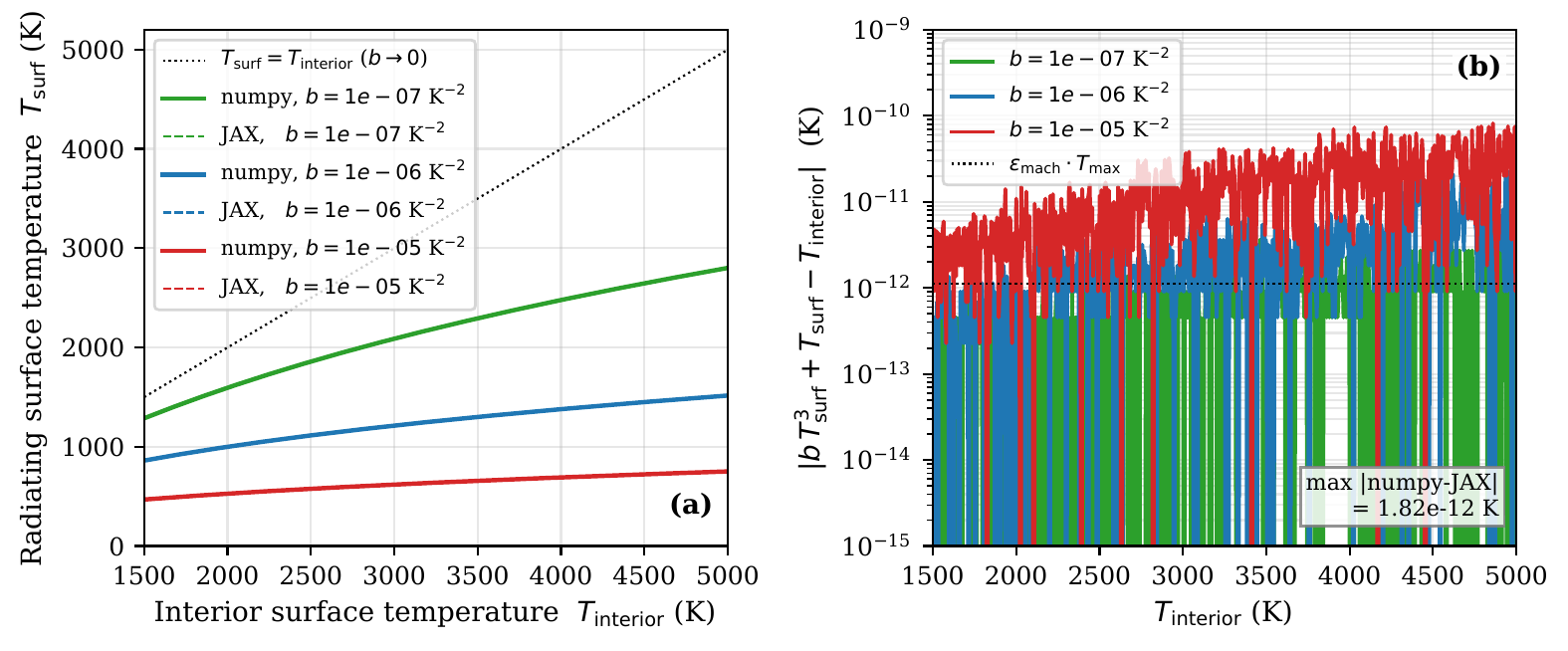
Figure 5. Surface-temperature correction from the upper-thermal-boundary-layer parameterisation (solver/boundary.py::_utbl_tsurf). The Cardano-formula solution to \(b x^3 + x - T_\mathrm{int} = 0\) recovers \(T_\mathrm{surf} < T_\mathrm{int}\) for the entire physical range and matches the cubic-equation residual to floating-point tolerance. Verifies the analytic surface boundary condition used when param_utbl = true.
Mesh tests (tests/test_jax_mesh_gravity_fallback.py)
Verify that when the external mesh file (eos_method = 2) supplies an eos_gravity column, the JAX path interpolates the per-node gravity profile onto the basic grid rather than broadcasting a single scalar.
Numpy <-> JAX RHS parity
Why this check exists. Aragog implements the right-hand side of the energy equation in both NumPy and JAX. The NumPy right-hand side is the reference implementation, and CVODE evaluates the compiled JAX right-hand side to integrate planet cooling. If the two paths differ in their rheology formulas or flux assembly, CVODE will integrate a different physical system than the reference equations. This test catches discrepancies in homologous temperature parameters on active-solid states (abe_solid_kappah_floor_0), where the JAX homologous perturbation probe produces relative differences in \([8.332 \times 10^{-3}, 1.0582 \times 10^{-2}]\) and fails the \(10^{-6}\) tolerance by a factor of 8332 to 10582 (\(> 8000\times\)). It catches missing plastic yielding in JAX on yielded states (abe_solid_yield_active), where disabling plastic yielding produces relative differences in \([8.529 \times 10^{-5}, 1.340 \times 10^{-4}]\) and fails tolerance by a factor of 85 to 134 (\(> 80\times\)). The default state set (abe_solid_default) does not show either fault. The test also catches a missing or weakened viscosity law: on abe_solid_kappah_floor_0 the law alone shifts the right-hand side by \([8.412 \times 10^{-3}, 1.0677 \times 10^{-2}]\), and the law-only guard requires \([4 \times 10^{-3}, 2 \times 10^{-2}]\) on the stored states and \([5 \times 10^{-3}, 2 \times 10^{-2}]\) on the live state (\(1.037 \times 10^{-2}\)). A law-cut mutant (rheology on with the rheology-off viscosity and mixing-length factor) gives 0 and fails it.
What it tests. With solid-state rheology enabled ([phase_solid.rheology] enabled = true), the right-hand side evaluates the rate of specific entropy change \(\dot{S} = \partial S/\partial t\) in both EntropyState.update (NumPy) and aragog.jax.phase.compute_fluxes (JAX). The test reads a stored sweep of 100 cooling states on three state sets (tests/reference/ssc_solver_wiring_benchmarks.json, made by tools/verification/generate_ssc_solver_wiring_benchmarks.py) and evaluates one live profile per set:
- Default configuration
cfg/abe_solid.toml: initial entropy \(S_\text{init} = 2900\text{ J/(kg K)}\), eddy-diffusivity floor \(\kappa_{h,\text{floor}} = 10.0\text{ m}^2/\text{s}\), and solid reference viscosity \(\eta_\text{solid} = 1.0\times 10^{21}\text{ Pa s}\). Solid rheology alters basic-node viscosity with solid blend weight \(1 - w(\phi) > 0\) at all 100 basic nodes, with effective viscosity \(\eta_\text{eff} = \eta_\text{diff}\) across all states (\(n_\text{states}(\eta_\text{eff} \ne \eta_\text{diff}) = 0\)). Rheology on vs off changes the right-hand side by \([8.101 \times 10^{-5}, 1.268 \times 10^{-3}]\). This change comes mostly from the solid-cell floor switch, not from the viscosity law: with rheology on, a fully solid cell gets no \(\kappa_{h,\text{floor}}\). - Active-solid Arrhenius variant
abe_solid_kappah_floor_0: \(S_\text{init} = 2500\text{ J/(kg K)}\), bottom entropy \(S_\text{bot} \in [1850, 2500]\text{ J/(kg K)}\), \(\kappa_{h,\text{floor}} = 0.0\text{ m}^2/\text{s}\), \(\eta_\text{solid} = 1.0\times 10^{18}\text{ Pa s}\), cohesion \(c = 1.0\times 10^7\text{ Pa}\), friction coefficient \(\mu = 0.1\), and maximum yield stress \(\tau_{y,\text{max}} = 1.0\times 10^8\text{ Pa}\). Homologous Arrhenius strengthening (\(\eta_\text{diff} \ge 10^{22}\text{ Pa s}\)) keeps Pass 1 convective flux below conductive flux through the column (\(f_\text{conv} < 0.5\)), sohas_lid = Falseand \(n_\text{nodes}(\eta_\text{eff} \ne \eta_\text{diff}) = 0\) in all 100 states while Arrhenius strengthening changes the RHS by \([8.412 \times 10^{-3}, 1.0677 \times 10^{-2}]\) (and \(0.99467\) along the integrated 100-yr trajectory on 60 basic nodes). - Yield-active state set
abe_solid_yield_active: warm sub-solidus interior \(S_\text{init} = 2150\text{ J/(kg K)}\), \(S_\text{bot} \in [1950, 2150]\text{ J/(kg K)}\), \(\Delta S \in [1620, 1820]\text{ J/(kg K)}\), \(\kappa_{h,\text{floor}} = 0.0\text{ m}^2/\text{s}\), \(\eta_\text{solid} = 3.0\times 10^{17}\text{ Pa s}\), \(c = 150.0\text{ Pa}\), \(\mu = 0.0\), and \(\tau_{y,\text{max}} = 1.0\times 10^8\text{ Pa}\). Pass 1 interior convection exceeds conduction (\(f_\text{conv} > 0.5\)) beneath a cold conductive upper boundary layer (has_lid = Truein all 100 states), generating driving stress \(\tau_{d,\text{lid}} \gg \tau_{y,\text{lid}} = 150\text{ Pa}\) so plastic yielding reduces \(\eta_\text{eff} < \eta_\text{diff}\) in 9 to 13 nodes in all 100 states. Yielding shifts the RHS relative to yield-off by \([8.529 \times 10^{-5}, 1.340 \times 10^{-4}]\) (median \(9.520 \times 10^{-5}\)). At the defaultmatprop_smooth_width = 0.01the blend gives the two solid nodes above the solidus the small two-phase thermal expansivity of the test tables, so their mixing-length diffusivity is near 0 with and without yield.
When single-phase thermal expansivity \(\alpha\) is harmonised between both paths (identity_alpha = True), abe_solid_kappah_floor_0 is unchanged because two-phase latent-blend node 98 (\(\phi = 0.5567\), \(\rho_\text{sol} < \rho_\text{liq}\)) uses alpha_mixed exclusively (flux_vs_rhs_diagnostic): a \(1\text{ ULP}\) jax.jit division rounding difference in negative unclamped \(\alpha_\text{mixed}\) (\(-3.559 \times 10^{-4}\text{ K}^{-1}\)) is amplified by cancellation in the smooth positivity clamp \(\alpha = \frac{1}{2}(a + \sqrt{a^2 + \epsilon_\alpha^2})\) (\(\epsilon_\alpha = 10^{-8}\text{ K}^{-1}\)) into a \(3.859 \times 10^{-7}\) relative shift in \(\alpha_{98} = 7.024 \times 10^{-14}\text{ K}^{-1}\) and a maximum relative right-hand side difference of \(4.584 \times 10^{-10}\) (median \(3.521 \times 10^{-16}\), interior heat-flux relative difference \(\le 5.095 \times 10^{-8}\); eager JAX at state 0 agrees with NumPy to \(8.066 \times 10^{-16}\)), asserted by the smoke test to within \(10^{-9}\) (\(2.18\times\) above \(4.584 \times 10^{-10}\), corresponding to \(2\text{ ULP}\) in unclamped \(\alpha_\text{mixed}\)). On abe_solid_yield_active and abe_solid_default, NumPy and JAX right-hand sides agree to floating-point round-off: \(\le 1.097 \times 10^{-15}\) (median \(2.823 \times 10^{-16}\), interior heat-flux relative difference \(\le 9.510 \times 10^{-14}\)) on abe_solid_yield_active, and \(\le 4.998 \times 10^{-15}\) (median \(2.127 \times 10^{-15}\), interior heat-flux relative difference \(\le 1.669 \times 10^{-14}\)) on abe_solid_default. With unharmonised single-phase \(\alpha\) where EntropyPhaseEvaluator interpolates the table directly and EntropyEOS_JAX evaluates the thermodynamic relation, differences remain within \(10^{-6}\) in all three state sets: \(\le 4.584 \times 10^{-10}\) (median \(5.509 \times 10^{-16}\), interior heat-flux relative difference \(\le 5.095 \times 10^{-8}\)) on abe_solid_kappah_floor_0, \(\le 1.255 \times 10^{-7}\) (median \(2.787 \times 10^{-8}\), interior heat-flux relative difference \(\le 2.987 \times 10^{-5}\)) on abe_solid_yield_active, and \(\le 4.998 \times 10^{-15}\) (median \(2.127 \times 10^{-15}\), interior heat-flux relative difference \(\le 1.669 \times 10^{-14}\)) on abe_solid_default. Live evaluation of a single profile verifies parity to within \(2.5 \times 10^{-13}\) relative error.
How we know the right answer. The NumPy and JAX implementations are independent code paths that derive from the same physical formulas. They must yield identical right-hand side rates within floating-point round-off.
Why it matters. The integrator relies on the JAX right-hand side for speed and differentiability. Discrepancies between NumPy and JAX would mean that model predictions depend on which code path is active.
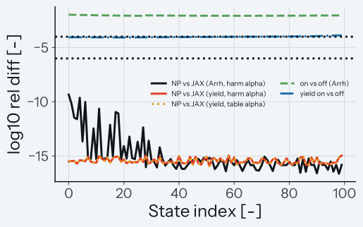
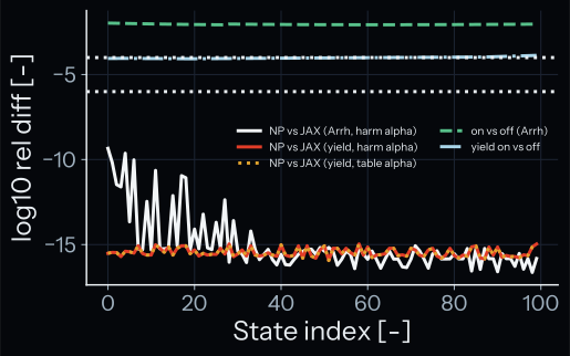
How to read the plot. The top row shows absolute differences between NumPy and JAX right-hand sides along mantle radius for the three state sets. The bottom row shows relative differences. The plot shows the stored 100-state sweep. A pass means that all points lie below the dashed tolerance line at \(10^{-6}\).
Test details
- Reference: NumPy
EntropySolver.dSdttwo-pass implementation onabe_solid_kappah_floor_0(s_init = 2500,kappah_floor = 0,viscosity_solid = 1e18),abe_solid_yield_active(s_init = 2150,kappah_floor = 0,viscosity_solid = 3e17,yield_stress_c = 150 Pa), and inert defaultabe_solid_default(s_init = 2900,kappah_floor = 10,viscosity_solid = 1e21). - Tolerance: \(\max_i |\dot{S}_{\text{NumPy}, i} - \dot{S}_{\text{JAX}, i}| / \max(|\dot{S}_{\text{NumPy}, i}|, 10^{-30}) \le 10^{-6}\) for all 100 states of each state set (asserted to \(\le 10^{-9}\) for harmonised active-solid RHS parity); active-solid on-vs-off relative difference in \([4 \times 10^{-3}, 2 \times 10^{-2}]\) (live state \([5 \times 10^{-3}, 2 \times 10^{-2}]\)) and yield-active yield-on vs yield-off relative difference \(\ge 10^{-5}\) at every state (live state \(\ge 5 \times 10^{-5}\)).
- Test id:
tests/test_rheology_solver_wiring_smoke.py::test_rhs_numpy_jax_parity_rheology_on - Command:
pytest tests/test_rheology_solver_wiring_smoke.py -k test_rhs_numpy_jax_parity_rheology_on(add--validation-plotsto write the plot pair)
Round-off perturbation spread with solid rheology
Why this check exists. Nonlinear rheology coupling can cause numerical instability where tiny floating-point round-off errors grow exponentially. This check verifies that microscopic initial perturbations do not cause divergent trajectory spreads during planetary thermal evolution.
What it tests. Five perturbed initial entropy profiles \(S_0^{(k)}(r) = S_0(r)\left(1 + k \cdot 10^{-12}\right)\) (\(k \in \{-2, -1, 0, +1, +2\}\)) are integrated forward for 100 years on the active-solid variant (s_init = 2500 J/(kg K), kappah_floor = 0.0 m^2/s, viscosity_solid = 1.0e18 Pa s) and the default cfg/abe_solid.toml (s_init = 2900 J/(kg K), kappah_floor = 10.0 m^2/s, viscosity_solid = 1.0e21 Pa s). The spread \(\Delta T(r) = \max_k T_k(r) - \min_k T_k(r)\) over all 100 basic nodes and all 99 staggered nodes measures trajectory sensitivity:
- Active-solid variant (
abe_solid_kappah_floor_0): solid rheology alters final temperatures by \(\max_r |T_\text{on}(r, t_\text{end}) - T_\text{off}(r, t_\text{end})| = 7.9874\text{ K}\) (\(T_\text{surf} = 482.079\text{ K}\) vs \(481.618\text{ K}\), relative difference at the surface \((T_\text{on,surf} - T_\text{off,surf}) / T_\text{off,surf} = 9.570 \times 10^{-4}\), relative difference normalized by peak mantle temperature \(\max_r |T_\text{on} - T_\text{off}| / \max_r T_\text{off} = 2.205 \times 10^{-3}\), RHS relative difference \(7.656 \times 10^{-2}\),visc_on != visc_offat all 100 basic nodes, and \(\kappa_{h,\text{on}} \ne \kappa_{h,\text{off}}\) at 60 basic nodes). Microscopic round-off perturbations yield maximum radial spread with rheology enabled of \(\max_r \Delta T_\text{on}(r) = 2.128 \times 10^{-5}\text{ K}\) (\(\Delta T_{\text{on,surf}} = 2.128 \times 10^{-5}\text{ K}\), \(\Delta T_{\text{on,cmb}} = 1.232 \times 10^{-9}\text{ K}\), \(\max_r \Delta T_{\text{on,stag}}(r) = 2.178 \times 10^{-5}\text{ K}\)) against \(\max_r \Delta T_\text{off}(r) = 1.232 \times 10^{-5}\text{ K}\) (\(\Delta T_{\text{off,surf}} = 1.232 \times 10^{-5}\text{ K}\), \(\Delta T_{\text{off,cmb}} = 1.255 \times 10^{-9}\text{ K}\), \(\max_r \Delta T_{\text{off,stag}}(r) = 1.433 \times 10^{-5}\text{ K}\)). The measured ratio \(\max_r \Delta T_\text{on} / \max_r \Delta T_\text{off}\) is \(1.727\); the deciding bounds are taken directly from the measurement, with the active-solid spread bounded by the \(3.5 \times 10^{-5}\text{ K}\) ceiling (\(1.64\times\) margin over the measured basic spread). - Default configuration
cfg/abe_solid.toml: solid rheology alters final basic temperatures by \(\max_r |T_\text{on}(r, t_\text{end}) - T_\text{off}(r, t_\text{end})| = 7.5340\text{ K}\), relative difference \(2.052 \times 10^{-3}\), RHS relative difference \(9.789 \times 10^{-2}\), with \(\max_r \Delta T_\text{on}(r) = 5.946 \times 10^{-7}\text{ K}\) and \(\max_r \Delta T_\text{off}(r) = 1.089 \times 10^{-6}\text{ K}\) (\(\Delta T_\text{surf} = 5.946 \times 10^{-7}\text{ K}\)). A run with the solid-cell floor switch and without the viscosity law changes the temperatures by \(7.485\text{ K}\). Adding the viscosity law to that run changes them by at most \(0.199\text{ K}\) more. Both are maxima over the radius, so they do not add up to \(7.534\text{ K}\).
How we know the right answer. Trajectories with rheology enabled must remain stable: their perturbation spread must not exceed the deciding bound set from the measured spread with a stated margin (\(3.5 \times 10^{-5}\text{ K}\) for active solid, \(2.0 \times 10^{-6}\text{ K}\) for default).
Why it matters. Unstable numerical behaviour causes planetary thermal evolution simulations to diverge or crash during multi-gigayear coupled runs.
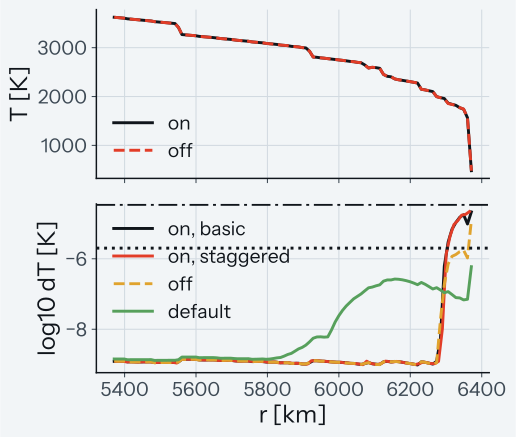
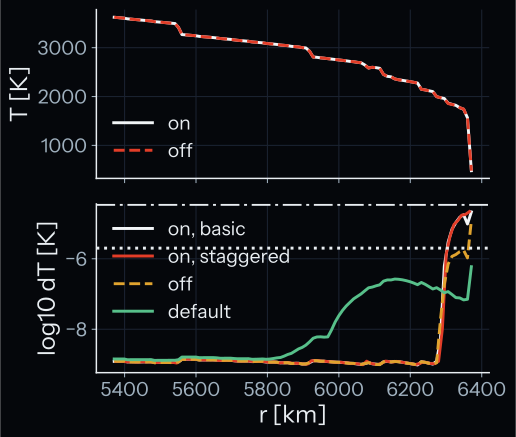
How to read the plot. The top panel shows end-time radial temperature profiles for rheology on and off on the active-solid variant. The bottom panel shows the radial perturbation spreads \(\Delta T(r)\) from the stored runs. A pass means the active-solid curves with rheology on (basic and staggered nodes) stay below the dash-dot line (\(3.5 \times 10^{-5}\text{ K}\)) and the default curve stays below the dotted line (\(2.0 \times 10^{-6}\text{ K}\)). The active-solid staggered curve comes closest to its bound: its margin is \(1.61\times\).
Test details
- Reference: 5 perturbed trajectories with
rheology.enabled = falseon the active-solid variant and defaultcfg/abe_solid.toml(tests/reference/ssc_solver_wiring_benchmarks.json). - Tolerance: \(\Delta T_\text{on}(r) \le 3.5 \times 10^{-5}\text{ K}\) (margin \(1.64\times\) over the measured basic spread \(2.128 \times 10^{-5}\text{ K}\) and \(1.61\times\) over the staggered spread \(2.178 \times 10^{-5}\text{ K}\)) on the active-solid variant and \(\Delta T_\text{on}(r) \le 2.0 \times 10^{-6}\text{ K}\) on default, with active-solid on-vs-off relative difference \(\ge 10^{-4}\).
- Test id:
tests/test_rheology_solver_wiring.py::test_perturbed_starts_spread - Command:
pytest tests/test_rheology_solver_wiring.py -k test_perturbed_starts_spread(add--validation-plotsto write the plot pair)
Two-pass solid rheology RHS cost
Why this check exists. Solid rheology calculations execute inside the innermost loop of the differential equation solver. Redundant lookups or repeated compilation would make simulations run slowly. This check counts kernel executions and reads the stored execution times to confirm that two-pass solid rheology adds only the expected kernel calls and that the recorded JAX wall-time ratio stays below 1.5.
What it tests. Enabling two-pass solid rheology (rheology.enabled = true) reuses the basic-node solidus temperature \(T_\text{sol}(P)\) already evaluated during phase lookup, skips staggered-node rheology viscosity via defer_rheology_viscosity = True (NumPy) and include_rheology = False (JAX), and calls the validation-free _core kernels directly inside the RHS. The test measures the call-count deltas live and reads the recorded wall times:
| Per-RHS item | Expected delta (on - off) |
Measured 'lid' delta (NumPy / JAX) |
Measured 'local' delta (NumPy / JAX) |
Difference ('lid' - expected) |
Reason |
|---|---|---|---|---|---|
| EOS lookups (solidus temperature) | 0 |
0 / 0 (5 - 5 / 6 - 6) |
0 / 0 |
0 |
T_sol(P) is cached on basic nodes during phase evaluation and reused without extra EOS lookups. |
compute_arrhenius_viscosity |
+2 |
+2 / +2 |
+1 / +1 |
0 |
In 'lid' mode: 1 vector call on \(N_b\) basic nodes in phase evaluation plus 1 scalar call at \((T_i, P_i)\) inside _compute_stagnant_lid_state_core (+2). In 'local' mode: 1 vector call on \(N_b\) basic nodes (+1). |
compute_yield_stress |
+2 |
+2 / +2 |
+1 / +1 |
0 |
In 'lid' mode: 1 vector call on \(N_b\) basic nodes in phase evaluation plus 1 scalar call at \(P_\text{lid,base}\) inside _compute_stagnant_lid_state_core (+2). In 'local' mode: 1 vector call on \(N_b\) basic nodes (+1). |
compute_stagnant_lid_state |
+1 |
+1 / +1 |
0 / 0 |
0 |
In 'lid' mode: 1 call per RHS between Pass 1 (unyielded probe) and Pass 2 (+1). In 'local' mode: active when stress_closure_mode == 'lid' (0). |
compute_effective_viscosity |
+1 |
+1 / +1 |
+1 / +1 |
0 |
1 vector call on \(N_b\) basic nodes in Pass 2 (+1 in both 'lid' and 'local' modes). |
viscous_mixing_length_factor |
+2 |
+2 / +2 |
+2 / +2 |
0 |
Relative to rheology.enabled = false (0 calls), Pass 1 (theta = None) and Pass 2 (theta = lid_state['theta'] in 'lid' mode, None in 'local' mode) each invoke _viscous_mixing_length_factor_core once, giving +2 calls per RHS in both NumPy and JAX. |
Each wall time is the minimum over 7 blocks of 1000 RHS evaluations on the 100-basic-node cfg/abe_solid.toml mesh (tests/reference/ssc_solver_wiring_benchmarks.json). The JIT-compiled JAX RHS wall-time ratio is \(1.293\times\) in 'lid' mode (\(789.02\,\mu\text{s}\) vs \(610.12\,\mu\text{s}\) per call) and \(1.125\times\) in 'local' mode (\(686.30\,\mu\text{s}\) vs \(610.12\,\mu\text{s}\) per call). The bound of \(1.5\times\) applies to this recorded ratio: the test and the generator's --check read it from the stored benchmark, so a slowdown of the code is detected only when the benchmark is regenerated. It is not a performance target. On the eager NumPy path, the two-pass RHS wall-time ratio is \(1.703\times\) in 'lid' mode (\(3087.04\,\mu\text{s}\) vs \(1813.03\,\mu\text{s}\)) and \(1.128\times\) in 'local' mode (\(2045.50\,\mu\text{s}\) vs \(1813.03\,\mu\text{s}\)). The generator's --check accepts NumPy ratios in \([0.8, 2.5]\). The test sets no bound on them.
How we know the right answer. The expected call numbers come directly from code design: Pass 1 calculates unyielded convection and Pass 2 applies lid geometry and yielding. Wall times are measured by the benchmark generator against identical runs with rheology disabled and stored in the JSON; the test reads them.
Why it matters. Coupled planetary simulations run tens of thousands of solver steps. In the recorded benchmark, the JAX ratio of \(1.293\) in 'lid' mode means that solid-state convection adds about \(29\%\) to the cost of the right-hand side. The ratios depend on the machine load at generation time. The test checks the recorded benchmark, so a new measurement needs a regeneration of the benchmark file.
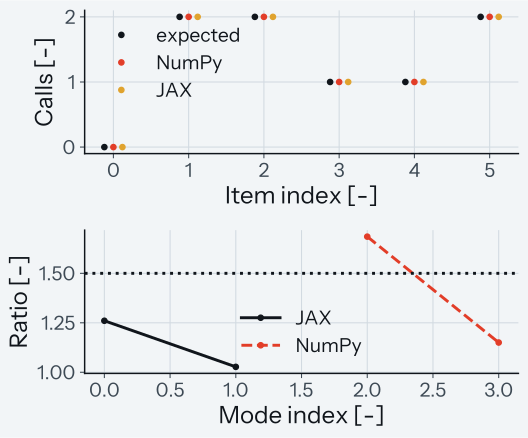
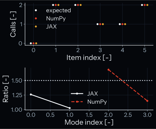
How to read the plot. The top panel shows call counts for the six kernel components. Points show expected deltas, measured NumPy deltas, and measured JAX deltas (matching across all components). The bottom panel shows wall-time ratios for JAX (solid line) and NumPy (dashed line). A pass means JAX ratios remain below the dotted guard line at \(1.5\).
Test details
- Reference:
rheology.enabled = falseper-RHS call counts and 1000-call wall time oncfg/abe_solid.toml. - Tolerance: per-RHS call-count deltas \((0, +2, +2, +1, +1, +2)\) in
'lid'mode and \((0, +1, +1, 0, +1, +2)\) in'local'mode on both NumPy and JAX; JIT-compiled JAX wall-time ratio \(\le 1.5\) (minimum over 7 blocks of 1000 calls, read from the stored benchmark). - Test id:
tests/test_rheology_solver_wiring.py::test_rhs_call_counts_and_cost - Command:
pytest tests/test_rheology_solver_wiring.py -k test_rhs_call_counts_and_cost(add--validation-plotsto write the plot pair)
Running the verification suite
The standalone suite uses pytest:
# Run the entire suite
pytest tests/

# Run a specific category
pytest tests/test_entropy_pytest.py
pytest tests/test_entropy_verification.py
pytest tests/test_jax_entropy.py

# Mark-filtered subsets
pytest -m unit tests/             # unit tests only
pytest -m smoke tests/            # smoke tests only
The JAX-path tests require jax and equinox to be installed; tests are skipped (not failed) when the optional dependencies are missing. Some tests also require the SPIDER-format EOS table directory; they look in ARAGOG_TEST_EOS_DIR, then in $FWL_DATA/aragog/spider_eos, then in a parity cache next to the repository (tests/conftest.py), and skip when none of them exists.
Physical constraints checked
The suite asserts the following physical invariants on every solver-driven test run:
- Temperature positivity. \(T > 0\) everywhere at all integration times. EOS lookups outside the table domain raise rather than silently extrapolating.
- Melt fraction bounds. \(0 \le \phi \le 1\) via the smooth-clip; the assertion runs at every staggered node.
- Pressure positivity and monotonicity. \(P(r)\) is positive and decreases monotonically from CMB to surface.
- Entropy gradient continuity. \(\partial S/\partial r\) and the resulting fluxes are \(C^0\) through the solidus and liquidus crossings (the smoothing functions enforce this).
- Energy conservation. Within the integrator tolerance, \(\Delta E_\mathrm{th}\) matches the time-integrated boundary fluxes plus internal heating sources.
- Mass conservation. Total mantle mass is preserved under gravitational separation and chemical mixing (the segregation flux is divergence-free in mass).
Phase-boundary rate controller verification
What this section checks
This section verifies the event-driven phase-boundary rate controller (phase_boundary_cap = "rate").
The controller regulates time steps in the CVODE solver near phase boundaries (solidus and liquidus) and during solid mantle cooling.
We verify that rate segmentation maintains temperature accuracy to \(1.3 \times 10^{-4}\text{ K}\) against a high-resolution reference (\(1\text{ yr}\) steps at rtol \(10^{-10}\)).
Tolerances in this section are given as the relative tolerance rtol.
The solver keeps the absolute tolerance atol at \(10^{-8}\) or above, in the unit of each state entry.
It multiplies atol by 10 when the mean melt fraction at the start of a call is at most 0.01.
A case states where it sets atol another way.
We also report the round-off envelope of the controller cases and verify non-stalling behavior during mantle solidification; 2 coupled PROTEUS cases compare runs with and without the rules of the controller.
The cases below evaluate accuracy, stiff-zone boundary landing, post-solidification stepping, and coupled behavior.
Accuracy of event-driven rate segmentation at phase boundaries
Why this check exists. Near phase boundaries, latent heat release causes sharp changes in effective heat capacity. If time steps are too large near a phase boundary, the numerical integrator incurs large local truncation errors or step rejections.
What it tests.
Four test cases (Cases A, B, C, D) cover two core boundary conditions and 16 to 24 nodes.
Cases A, C and D start in the mushy zone; Case B starts \(230\text{ J/(kg K)}\) above the liquidus.
Cases A, B and D use the smoothing width \(w = 0.01\), Case C uses \(w = 0\).
The test compares the temperature profile \(T(r)\) from phase_boundary_cap = "rate" at rtol \(10^{-8}\) against a high-resolution reference (phase_boundary_cap = "fixed" at rtol \(10^{-10}\), with a \(1\text{ yr}\) ceiling on max_step in every CVODE solve).
How we know the right answer.
A \(1\text{ yr}\) ceiling on max_step at rtol \(10^{-10}\) resolves the phase boundaries.
The rate run at rtol \(10^{-10}\) ends within \(2.1 \times 10^{-6}\text{ K}\) of this reference in every case. In Cases A and C the end temperatures are equal.
Why it matters. Accurate temperatures near phase boundaries set the timing and depth of magma ocean crystallization in planetary evolution models.
Test details
- Reference: \(1\text{ yr}\) ceiling on
max_stepat rtol \(10^{-10}\) - Tolerance: \(\max_i |T_{\text{rate}, 10^{-8}, i} - T_{\text{fixed}, 10^{-10}, i}| \le 1.3 \times 10^{-4}\text{ K}\) (observed: Case A \(6.91 \times 10^{-6}\text{ K}\), Case B \(2.92 \times 10^{-5}\text{ K}\), Case C \(1.04 \times 10^{-5}\text{ K}\), Case D \(2.83 \times 10^{-5}\text{ K}\))
- Test id: V1 (rate segmentation accuracy): the command below; no pytest case runs it
- Command:
ARAGOG_TEST_EOS_DIR=... python tools/verification/run_phase_boundary_cap_accuracy.py --check
Stiff-zone boundary landing under slow cooling
Why this check exists. When a cell cools slowly near the boundary, its cooling rate \(|\dot{S}|\) can approach zero while the distance to the boundary remains small. Without a floor on the effective progress distance, the step cap could collapse to the \(1\text{ yr}\) minimum step bound, causing many tiny steps.
What it tests.
A 12-node column on the CI test table cools for \(15\,000\text{ yr}\) under a prescribed surface flux \(F = 20\text{ W/m}^2\), with matprop_smooth_width \(= 0\), so that the stiff-zone half-width is \(\delta = 10\text{ J/(kg K)}\).
Cells 4 and 5 start \(11\) and \(12.5\text{ J/(kg K)}\) above the solidus, just outside the stiff zone; the other cells start \(15\text{ J/(kg K)}\) below it, off the edge of the stiff zone.
This case checks the step controller only; it is not a model of a planet.
The flux is chosen for the entropy range of the CI test table.
The stiff-zone landing rule (\(d_{\text{eff}} = \max(d_{\text{near}}, 0.5\,\delta)\)) sets the step while these cells land on the solidus.
The tool counts the slow-landing segments: segments whose step is set by a cell closer than \(0.5\,\delta\) to a boundary, with its rate (floored at the mass-weighted mean rate) below \(0.05\,\delta\) per year.
How we know the right answer.
The reference solve uses \(1\text{ yr}\) steps at rtol \(10^{-10}\) with a physical atol of at most \(10^{-10}\) (set through solver._atol_sf).
The error is the largest temperature difference to the reference at the end.
Five starts with relative round-off perturbations of \(10^{-12}\) give the round-off envelope \(\Delta_{\text{pert}}\), the largest difference to the unperturbed run.
The error and \(\Delta_{\text{pert}}\) are separate numbers: the error must stay below the bound.
Why it matters. Slow cooling near the solidus occurs in long runs. Without the distance floor, a cell that starts a segment almost on its solidus limits the step to \(1\text{ yr}\); the known limit near \(96\text{ Myr}\) shows one such interval in a long run.
Test details
- Reference: \(1\text{ yr}\) steps at rtol \(10^{-10}\) and physical atol at most \(10^{-10}\); 5 round-off starts
- Tolerance: \(\|T_{\text{rate}}^{(0)} - T_{\text{fixed}, 10^{-10}}\|_\infty \le 1.3 \times 10^{-4}\text{ K}\) (observed: \(1.16 \times 10^{-5}\text{ K}\), envelope \(\Delta_{\text{pert}} = 4.4 \times 10^{-9}\text{ K}\); 224 steps in 11 segments, 4 of them slow landings; the reference takes 15002 steps). With
--checkthe case also fails above 250 steps: without the distance floor it takes 272 - Test id: V3-R3 (slow landing at the solidus): the command below;
tests/test_step_cap_validation_runs.py::test_v3_rate_run_counts_its_segments_inside_the_step_ceiling[v3_r3]runs the rate run at \(m = 0\) - Command:
ARAGOG_TEST_EOS_DIR=... python tools/verification/run_step_cap_validation.py --case v3_r3 --check
Sub-solidus upper-bound relaxation and tolerance tightening
Why this check exists. Once the entire mantle cools below the solidus, no phase boundary lies ahead in the cooling direction. Imposing a \(100\text{ yr}\) step ceiling on sub-solidus cooling slows down computation. Removing the \(100\text{ yr}\) ceiling without tightening tolerances could degrade solution accuracy.
What it tests.
A 12-node column on the CI test table cools for \(200\,000\text{ yr}\) under a prescribed surface flux \(F = 200\text{ W/m}^2\), with matprop_smooth_width \(= 0\).
Every cell starts at the solidus entropy of the top cell plus \(5\text{ J/(kg K)}\): the top cell starts above its solidus, the deeper cells start \(306\) to \(485\text{ J/(kg K)}\) below theirs.
This case checks the step controller only; it is not a model of a planet.
The flux is chosen so that every cell stays inside the entropy range of the CI test table.
A segment that starts with all cells at or below the solidus has no upper step bound; it ends where a cell passes its solidus.
Every segment that starts with all cells at or below the solidus uses the tighter tolerances \(\mathtt{rtol} \le 10^{-9}\) and \(\mathtt{atol} \le 10^{-8}/\text{scale}\).
How we know the right answer. The reference and the round-off starts are those of the case above. The run must stay within \(1.3 \times 10^{-4}\text{ K}\) of the reference.
Why it matters. Solid-state cooling after the magma ocean covers billions of years. The relaxed step bound lets such runs finish in reasonable time; this case checks that the error stays inside the tolerance below. The physical case for this regime is the full solidification check: a 100-node mantle on the PALEOS low-temperature table.
Not checked. A stiff-zone cell that cools at a segment start and heats inside a relaxed segment. A segment that starts with a cell heating within \(\delta\) of the solidus. No segment of this case starts that way; Heated sub-solidus segment that ends at the solidus checks one that reaches the solidus.
Test details
- Reference: \(1\text{ yr}\) steps at rtol \(10^{-10}\) and physical atol at most \(10^{-10}\); 5 round-off starts
- Tolerance: \(\|T_{\text{rate}}^{(0)} - T_{\text{fixed}, 10^{-10}}\|_\infty \le 1.3 \times 10^{-4}\text{ K}\) (observed: \(7.54 \times 10^{-5}\text{ K}\) in 1031 steps and 12 segments, 11 of them sub-solidus; the reference takes 200001 steps; envelope \(\Delta_{\text{pert}} = 1.07 \times 10^{-6}\text{ K}\), where 2 of the 5 starts take one sub-solidus segment less and 1028 steps). With
--checkthe case also fails above 1500 steps or without a segment with an infinite step bound: without the distance floor it takes 2669 steps, with the \(100\text{ yr}\) ceiling kept 2081 steps and no infinite bound - Test id: V3-R4 (sub-solidus relaxation): the command below;
tests/test_step_cap_validation_runs.py::test_v3_rate_run_counts_its_segments_inside_the_step_ceiling[v3_r4]runs the rate run at \(m = 0\) - Command:
ARAGOG_TEST_EOS_DIR=... python tools/verification/run_step_cap_validation.py --case v3_r4 --check
Heated sub-solidus segment that ends at the solidus
Why this check exists. A segment that starts with every cell at or below the solidus has no \(100\text{ yr}\) step ceiling, and the step rule is read only at the start of a segment. A cell that heats and passes its solidus inside such a segment would melt with the large step ceiling and the tight sub-solidus tolerances. Without the solidus root this case fails: the run stays one segment without the \(100\text{ yr}\) ceiling.
What it tests.
A 12-node column (11 cells) on the CI test table is heated through its surface by \(400\text{ W/m}^2\) for \(10\,000\text{ yr}\), with convective_threshold \(= 0\).
The default matprop_smooth_width \(= 0.01\) sets the stiff-zone half-width \(\delta = 251.8\text{ J/(kg K)}\).
The top cell starts \(2\text{ J/(kg K)}\) below its solidus, closer than \(0.5\,\delta\); the other cells start \(300\text{ J/(kg K)}\) below theirs.
This case checks the step controller only; it is not a model of a planet.
The first segment must have a step ceiling (max_step) above \(100\text{ yr}\) and end at the solidus root, an event that CVODE watches during the segment.
The next segment starts with the top cell just above its solidus, so its step ceiling is at most \(100\text{ yr}\) and it uses the caller's tolerances.
The case checks this segment structure; its largest CVODE step before the solidus is \(135\text{ yr}\), so the accuracy of much longer steps is the next case.
How we know the right answer.
The reference solve uses \(1\text{ yr}\) steps (phase_boundary_cap = 'fixed') at rtol \(10^{-10}\) and a physical atol of \(10^{-10}\).
A \(1\text{ yr}\) step at rtol \(10^{-10}\) resolves the solidus crossing on its own, so the reference does not depend on the step controller.
The error is the largest temperature difference to the reference over the output times that both runs share.
Five starts with relative round-off perturbations of \(10^{-12}\) give the round-off envelope \(\Delta_{\text{pert}}\), the largest difference of a perturbed run from the unperturbed run.
The bound is the \(1.3 \times 10^{-4}\text{ K}\) of the sub-solidus case above.
Why it matters. A cooled mantle can heat and melt again; once a cell melts, the solver must return to the \(100\text{ yr}\) ceiling. The temperatures alone do not show it: without the solidus root this case still meets the bound at the end (\(9.75 \times 10^{-5}\text{ K}\)), so the segment structure is checked by itself.
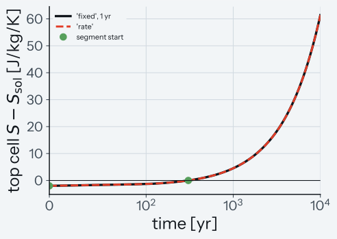
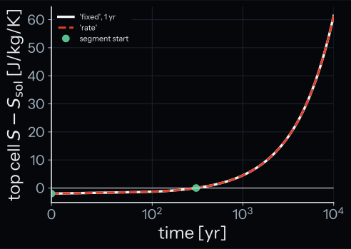
How to read the plot. The horizontal axis is time in years, linear up to \(100\text{ yr}\) and logarithmic above. The vertical axis is the entropy of the top cell minus its solidus entropy; the top cell is partly molten above the line at zero. The solid line is the \(1\text{ yr}\) reference, the dashed line the rate run; the dots are the segment starts. The first dot lies \(2\text{ J/(kg K)}\) below the line at zero; the second lies on it, where the solidus root ends the first segment. A pass shows the two lines on top of each other and a segment start at zero; a run without the root also gives two such lines, but no dot at zero.
Known limit: start gap and heat flux. Over start gaps of 0, 0.5, 2 and \(10\text{ J/(kg K)}\) and heat fluxes of 200 and \(800\text{ W/m}^2\), the error over time is \(4.67 \times 10^{-5}\) to \(1.39 \times 10^{-4}\text{ K}\). At a start gap of \(0.5\text{ J/(kg K)}\) it is above the bound: \(1.39 \times 10^{-4}\text{ K}\) at \(2659\text{ yr}\), long after the solidus root at \(76.5\text{ yr}\) (at the end \(8.27 \times 10^{-5}\text{ K}\)). The error comes from the mushy segment after the root, which runs at the caller's rtol \(10^{-8}\), as every mushy segment does. The code without the solidus root integrates this whole call at rtol \(10^{-9}\), because its only segment starts sub-solidus.
Known limit: a heated cell that stays below the solidus. With the top cell 80, 100 or 120 J/(kg K) below its solidus, the run stays sub-solidus and the error over time is \(2.90 \times 10^{-4}\), \(3.44 \times 10^{-4}\) and \(3.52 \times 10^{-4}\text{ K}\). The code without the relaxed step ceiling gives the same end temperatures, so the ceiling does not cause these errors. The sub-solidus tolerance rtol \(10^{-9}\) does: with the rate run at rtol \(10^{-10}\) the error at 100 J/(kg K) falls to \(2.74 \times 10^{-5}\text{ K}\).
Not checked. The same case on the PALEOS low-temperature table; this case uses the CI test table.
Test details
- Reference: \(1\text{ yr}\) steps at rtol \(10^{-10}\) and a physical atol of \(10^{-10}\); 5 round-off starts \(S_0 (1 + m \cdot 10^{-12})\), \(m = -2, \dots, 2\)
- Tolerance: \(\max_t \|T_{\text{rate}} - T_{\text{fixed}, 10^{-10}}\|_\infty \le 1.3 \times 10^{-4}\text{ K}\) over the shared output times (observed: \(7.60 \times 10^{-5}\text{ K}\), \(5.83 \times 10^{-5}\text{ K}\) at the end; 118 steps in 2 segments; the first segment has a step ceiling of \(1915\text{ yr}\) and ends at the solidus root at \(304.9\text{ yr}\); the reference takes 10002 steps; envelope \(\Delta_{\text{pert}} = 5.9 \times 10^{-9}\text{ K}\))
- Test id:
tests/test_phase_boundary_cap.py::test_rate_mode_ends_a_subsolidus_segment_at_the_solidus - Command:
ARAGOG_TEST_EOS_DIR=... pytest tests/test_phase_boundary_cap.py -k test_rate_mode_ends_a_subsolidus_segment_at_the_solidus(add--validation-plotsto write the plot pair); the numbers of this case and of its known limits:python tools/verification/run_subsolidus_heating_cases.py --case heated --check,--case sweepand--case limit
Long steps while a cell heats to the solidus
Why this check exists. The relaxed step ceiling saves time only when CVODE takes steps far above \(100\text{ yr}\) while a cell heats towards its solidus. In the case above the largest such step is \(135\text{ yr}\), so it does not check the accuracy of long steps. This case does: it fails if a step of at least \(1000\text{ yr}\) is not taken before the solidus, or if the error leaves the bound.
What it tests.
A 12-node column (11 cells) on the CI test table starts at one temperature, with the top cell \(2\text{ J/(kg K)}\) below its solidus and every other cell further below its own.
Internal heating of \(10^{-8}\text{ W/kg}\) warms every cell, the surface is insulated, and the run lasts \(15\,000\text{ yr}\), with convective_threshold \(= 0\) and the default matprop_smooth_width.
This case checks the step controller only; it is not a model of a planet.
CVODE must take a step of at least \(1000\text{ yr}\) before the top cell reaches its solidus; then the solidus root ends the segment, and the next segment has a step ceiling of at most \(100\text{ yr}\).
The code that keeps the \(100\text{ yr}\) ceiling for a heating cell within \(\delta\) of the solidus cannot take such a step.
How we know the right answer. The reference and the bound are those of the case above: \(1\text{ yr}\) steps at rtol \(10^{-10}\) and a physical atol of \(10^{-10}\), and \(1.3 \times 10^{-4}\text{ K}\) at every output time that both runs share.
Why it matters. In a long run the speed-up of a solid mantle comes from such long steps, also when a cell heats slowly towards its solidus.
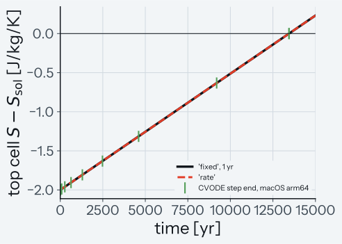
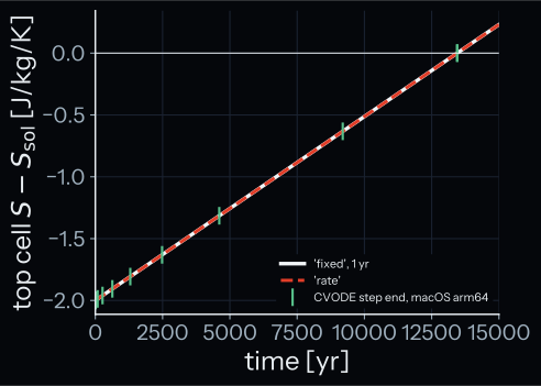
How to read the plot.
The horizontal axis is time in years; the vertical axis is the entropy of the top cell minus its solidus entropy.
The solid line is the \(1\text{ yr}\) reference and the dashed line the rate run.
The short vertical marks are the ends of the CVODE steps before the top cell reaches its solidus at the line at zero.
The step ends depend on the platform round-off (12 marks on macOS arm64, 13 on the Linux CI runner), so the marks come from a stored macOS arm64 run in tests/validation/data/rate_cap_subsolidus_long_steps.json; the test checks the long step on every platform.
A pass shows the two lines on top of each other and marks several thousand years apart.
Test details
- Reference: \(1\text{ yr}\) steps (
phase_boundary_cap = 'fixed') at rtol \(10^{-10}\) and a physical atol of \(10^{-10}\) - Tolerance: \(\max_t \|T_{\text{rate}} - T_{\text{fixed}, 10^{-10}}\|_\infty \le 1.3 \times 10^{-4}\text{ K}\) over the shared output times, and a step of at least \(1000\text{ yr}\) before the solidus (observed: \(4.69 \times 10^{-7}\text{ K}\), \(2.61 \times 10^{-7}\text{ K}\) at the end; largest step before the solidus \(4589\text{ yr}\); solidus root at \(13\,448\text{ yr}\); 28 steps against 15002 for the reference; round-off envelope \(\Delta_{\text{pert}} = 2.2 \times 10^{-6}\text{ K}\) over 5 starts \(S_0 (1 + m \cdot 10^{-12})\), so the error lies inside the round-off spread)
- Test id:
tests/test_phase_boundary_cap.py::test_rate_mode_takes_long_steps_while_a_cell_heats_to_the_solidus - Command:
ARAGOG_TEST_EOS_DIR=... pytest tests/test_phase_boundary_cap.py -k test_rate_mode_takes_long_steps_while_a_cell_heats_to_the_solidus(add--validation-plotsto write the plot pair); the numbers:python tools/verification/run_subsolidus_heating_cases.py --case long_steps --check; the stored marks: add--step-ends tests/validation/data/rate_cap_subsolidus_long_steps.json
Full solidification without solver stalling
Why this check exists.
A 100-node run must stay cheap through the slow final stages of solidification.
With stagnant-lid rheology (rheo_on), deep cells stay close to the phase boundary for hundreds of millions of years.
If the controller ties the step to their small distance from the boundary, the step size collapses.
Without rheology (rheo_off), the mantle is fully solid after about \(0.1\text{ Myr}\).
A \(100\text{ yr}\) step ceiling would then need about \(10^6\) steps to reach \(107.575\text{ Myr}\).
The code without the rules near and below the solidus stops after \(10^5\) steps in one output interval (solver.max_steps).
Those 2 runs store their time once every 1000 right-hand-side evaluations, and each stops after its last stored time.
The check uses these last stored times as stall points: \(83.684\text{ Myr}\) with rheology and \(107.575\text{ Myr}\) without it.
What it tests.
A 100-node mantle on the PALEOS low-temperature equation of state tables cools from \(S_0 = 3165.90\text{ J/(kg K)}\) under a grey-body surface (\(T_{\text{eq}} = 273\text{ K}\)), once with stagnant-lid rheology (rheo_on, until full solidification, \(\phi_{\max} = 0\)) and once without it (rheo_off, to \(120\text{ Myr}\)).
How we know the right answer. Each run must pass its stall point and reach \(\phi_{\max} = 0\) with status 0. Its entropy must stay inside the table.
Why it matters. Long planetary evolution runs require robust integration from magma ocean through complete mantle solidification into solid-state convection.
Known limit.
The rheo_on run stops at full solidification; the rheo_off run stops at \(120\text{ Myr}\).
Neither run integrates to \(10^9\text{ yr}\).
The rheo_on run installs the JAX CVODE factory, as coupled PROTEUS runs do.
Known limit: accuracy near \(96\text{ Myr}\).
In the rheo_on run, the second cell from the top sits about \(10^{-10}\text{ J/(kg K)}\) below its solidus near \(96\text{ Myr}\) while it still cools.
Without the rules near and below the solidus, this small distance limits the step to \(1\text{ yr}\).
The stiff-zone landing rule floors the distance at \(0.5\,\delta\), so the step can grow to \(100\text{ yr}\).
From \(96.08\) to \(96.54\text{ Myr}\) the run takes \(4598\) steps instead of \(459\,767\).
At rtol \(= 10^{-9}\), the temperature at the end of this interval then differs by up to \(8.4 \times 10^{-4}\text{ K}\) from the run without these rules (at rtol \(10^{-9}\) and \(10^{-10}\) that run gives the same state bitwise). The two runs end \(9.3\text{ yr}\) apart; the comparison moves one end state to the time of the other with its own \(\mathrm{d}S/\mathrm{d}t\) (first- and second-order steps agree; without the shift the difference is \(6.1 \times 10^{-4}\text{ K}\)).
At rtol \(= 10^{-10}\) to \(10^{-12}\) (atol stays at \(10^{-7}\) by the convention above), the result changes by less than \(5.5 \times 10^{-7}\text{ K}\) and stays within \(4.3 \times 10^{-6}\text{ K}\) of the run without these rules.
The difference at \(10^{-9}\) is thus an integration error of the larger steps.
From \(96\) to \(99\text{ Myr}\), the run stays \(2.2\) to \(2.8 \times 10^{-3}\text{ K}\) from the mean of 5 runs at rtol \(= 10^{-10}\).
This is up to 2.9 times the spread of those 5 runs.
The offset is already \(2.8 \times 10^{-3}\text{ K}\) at \(96.08\text{ Myr}\), before the interval above.
At \(100.9\) and \(103.5\text{ Myr}\) the offset is inside the spread again.
Test details
- Reference: Stall points at the last stored times, \(83.684\text{ Myr}\) (
rheo_on) and \(107.575\text{ Myr}\) (rheo_off) - Tolerance: Each run passes its stall point and reaches \(\phi_{\max} = 0\) with status 0; the entropy stays inside the table
- Test id: V4 (full solidification): the commands below;
tests/test_step_cap_validation_runs.py::test_v4_rheo_on_runs_with_the_jax_factoryruns \(10\text{ yr}\) of therheo_onpath on the CI test table - Command:
python tools/verification/run_step_cap_validation.py --case v4_rheo_off --eos-dir <PALEOS low-T table directory> --check; the same with--case v4_rheo_on
Coupled planetary evolution under super-solidus conditions
Why this check exists. Coupling Aragog to the PROTEUS framework exchanges heat fluxes and boundary temperatures with the atmosphere model (JANUS). The rules of the controller act only in a call that arms the rate cap: a call that starts within the arming margin of the liquidus or the solidus, or in the mushy band. A coupled run that stays far above the liquidus must therefore give the same state with and without the rules.
What it tests.
PROTEUS couples Aragog and JANUS for 5 iterations from \(T_{\text{surf}} = 4000\text{ K}\) (the PROTEUS default of planet.tsurf_init).
The run stays above the solidus (\(\Phi_{\text{global}} = 1\) at the end).
How we know the right answer. The end state is bitwise equal to that of the same run without the rules of the controller near and below the solidus. This holds for the 9 tracked helpfile columns and for the staggered temperature and entropy profiles.
Why it matters. This case checks that a coupled run above the liquidus gives the same state with and without the rules.
Not checked. How many calls of this run arm the rate cap (not measured). A coupled run that cools through the liquidus, where the stiff-zone landing rule acts above the solidus (see the effect on the second accuracy case in the energy equation).
Test details
- Reference: The same coupled run with the Aragog commit without the rules of the controller near and below the solidus
- Tolerance: Bitwise equality of
Time,T_magma,T_surf,F_int,F_atm,Phi_global,M_mantle_liquid,M_mantle_solid,R_intand the staggered profiles - Test id: V5 (coupled run above the solidus): the commands below;
tests/test_compare_v5_runs.pytests the comparison - Config:
tools/verification/data/v5_aragog_janus.toml; its header records the PROTEUS commit of the case and the Aragog commit of the second run - Command:
proteus start --offline -c tools/verification/data/v5_aragog_janus.tomlwith this Aragog, then again with the Aragog commit of the config header, each run with its own output folder (setparams.out.pathin a copy of the config); thenpython tools/verification/compare_v5_runs.py --case v5 RUN MAIN. The script checks both versions against the config header and writes them to its result file
Coupled planetary evolution crossing the solidus into the solid regime
Why this check exists. When a coupled PROTEUS planet cools below the critical melt fraction into the solid regime, every cell of the interior ends up at or below its solidus. The coupled run must cross the solidus and execute solid-state steps smoothly.
What it tests. PROTEUS couples Aragog and CALLIOPE from the mushy zone (\(T_{\text{surf}} = 1750\text{ K}\)). The run stops at the 3rd coupling step with a global melt fraction of zero.
How we know the right answer.
A strict reference integrates every CVODE call of the run with a \(1\text{ yr}\) ceiling on max_step at rtol \(10^{-10}\) and a physical atol of \(10^{-10}\), so its step size and tolerances do not depend on the step controller (its segment roots still split each call).
The check compares the error of the run against that reference with the error of the same run on the Aragog code without the rules of the controller near and below the solidus.
It uses 11 columns: the 9 tracked helpfile columns and the staggered temperature and entropy profiles.
A column passes when the error of the run is not larger than that of the run without the rules, plus a round-off floor.
The floor is the largest change of a column when either run starts from \(S_0 (1 \pm 10^{-12})\).
Why it matters. This case measures the cost of the rules at the solidus in a coupled run: on 4 of the 11 columns the error of the run is larger than without the rules (see the known limit), and the comparison tool exits with status 1.
Known limit.
The run passes on 7 columns and fails on 4: T_magma, T_surf, F_int and F_atm.
Its T_magma error is \(1.01 \times 10^{-3}\text{ K}\), against \(7.5 \times 10^{-4}\text{ K}\) without the rules; the gap of \(2.6 \times 10^{-4}\text{ K}\) is 7.8 times the round-off floor of \(3.3 \times 10^{-5}\text{ K}\).
The fluxes show the same ratio: F_int \(4.14 \times 10^{-2}\) against \(3.07 \times 10^{-2}\text{ W/m}^2\).
For the staggered profiles the error of the run is smaller: \(2.6 \times 10^{-3}\text{ K}\) against \(3.3 \times 10^{-3}\text{ K}\) in temperature.
The run takes 5856 CVODE steps, the run without the rules 5336.
At rtol \(10^{-11}\) the reference moves by \(3.4 \times 10^{-5}\text{ K}\) in T_magma, and the 4 columns still fail.
Which rule causes the gap in this run is not measured; near \(96\text{ Myr}\) in the full solidification check, a gap of this kind comes from larger steps next to a cell close to its solidus.
Test details
- Reference: \(1\text{ yr}\) ceiling on
max_stepat rtol \(10^{-10}\) and physical atol \(10^{-10}\) in every CVODE call; the same coupled run with the Aragog commit without the rules of the controller near and below the solidus; 4 round-off runs for the floor - Tolerance: On each of the 11 columns, the error against the reference is not larger than that of the run without those rules plus the round-off floor (observed: 7 columns pass;
T_magma,T_surf,F_intandF_atmfail, see the known limit) - Test id: V5b (coupled run through the solidus): the commands below;
tests/test_compare_v5_runs.pytests the comparison andtests/test_step_cap_validation_tool.pythe driver - Config:
tools/verification/data/v5b_aragog_calliope.toml; its header records the PROTEUS commit of the case and the Aragog commit of the second run - Command:
python tools/verification/run_v5b_proteus.py --output-dir RUNwith this Aragog,--reference --output-dir REFfor the reference,--s0-eps=1e-12 --output-dir RUN_Pand--s0-eps=-1e-12 --output-dir RUN_Mfor the floor; the same runsMAIN,MAIN_PandMAIN_Mwith the Aragog commit of the config header; thenpython tools/verification/compare_v5_runs.py --case v5b RUN MAIN --reference REF --floor RUN_P RUN_M MAIN_P MAIN_M
-
T. Ruedas, Radioactive heat production of six geologically important nuclides, Geochemistry, Geophysics, Geosystems, 18, 3530–3541, 2017. SciX. ↩
-
B. Jacobsen, Q.-Z. Yin, F. Moynier, Y. Amelin, A. N. Krot, K. Nagashima, I. D. Hutcheon, H. Palme, 26Al-26Mg and 207Pb-206Pb systematics of Allende CAIs: Canonical solar initial 26Al/27Al ratio reinstated, Earth and Planetary Science Letters, 272, 353-364, 2008. SciX. ↩
-
H. Tang, N. Dauphas, Abundance, distribution, and origin of 60Fe in the solar protoplanetary disk, Earth and Planetary Science Letters, 359-360, 248-263, 2012. SciX. ↩
-
W. F. McDonough, S.-s. Sun, The composition of the Earth, Chemical Geology, 120, 223-253, 1995. SciX. ↩