Orbit and tides¶

This tutorial demonstrates how to use PROTEUS to model the orbital and tidal evolution of a planet with a satellite. It covers the setup of the planet-satellite system, the configuration of tidal parameters, and the execution of simulations to study the effects of tides on planetary orbits.

Prerequisites¶

Full PROTEUS installation with AGNI, SOCRATES, and Obliqua compiled
FWL_DATA and RAD_DIR environment variables set
Spectral files downloaded (proteus get spectral -n Dayspring -b 48)
Solar spectrum downloaded (proteus get stellar)
Interior data downloaded, including the PALEOS EOS tables for the structure solver (proteus get interiordata --config-path input/tutorials/tutorial_earth.toml)

Reference data is also fetched automatically when proteus start runs without the --offline flag, so the download commands above are only required for offline use.

Physical setup¶

The physical setup for the orbit and tides tutorial involves defining the properties of the planet and its satellite. For the satellite a data file called tutorial_earth_moon.json is included in the input/tutorials/ directory relative to the PROTEUS root directory. The data file must be a JSON file with the following structure:

{
    "omega": 1.0e-06,       // Orbital frequency in rad/s
    "axial": 1.0e-06,       // Axial rotation frequency in rad/s
    "ecc": 0.1,             // Orbital eccentricity
    "sma": 1.82e7,          // Semi-major axis in meters
    "S_mass": 6e24,         // Mass of the central body in kg
    "density": [            // Radial density profile in kg/m^3
        7822.0,             // Iron core density
        3500.0,             // Solid mantle density
        3500.0              // Molten crust density
    ],
    "radius": [             // Radial radius profile in meters
        480000.0,           // Radius of the iron core in meters
        995613.0,           // Radius of the solid mantle in meters
        1650000.0           // Radius of the molten crust in meters (i.e. the surface)
    ],
    "visc": [               // Viscosity profile in Pa.s
        1e22,               // Viscosity of the solid mantle in Pa.s
        1e2                 // Viscosity of the molten crust in Pa.s
    ],
    "shear": [              // Shear modulus profile in Pa
        65857968278.256905, // Shear modulus of the solid mantle in Pa
        10.0                // Shear modulus of the molten crust in Pa
    ],
    "bulk": [               // Bulk modulus profile in Pa
        147739735943.7933,  // Bulk modulus of the solid mantle in Pa
        1000000000.0        // Bulk modulus of the molten crust in Pa
    ],
    "phi": [                // Porosity profile (dimensionless)
        0.0,                // Porosity of the solid mantle (dimensionless)
        1.0                 // Porosity of the molten crust (dimensionless
    ]
}

The specific values provided here reflect a partially molten Moon, with a fluid iron core, a solid mantle, and a partially molten crust. Although we do not require the orbital parameters for this test case, we still need to provide them in the data file. The values provided here are arbitrary and do not affect the tidal response calculations.

Running the simulation¶

conda activate proteus
mkdir -p output/tutorial_earth_moon
proteus start -c input/tutorials/tutorial_earth_moon.toml

Add --offline to skip the reference-data check on later runs; the first run must be able to download any missing data (or download it beforehand, see the prerequisites above).

Monitor progress with tail -f output/tutorial_earth_moon/proteus_00.log (the log appears once PROTEUS has initialized).

Runtime

This run takes roughly 20 minutes depending on hardware. A fine excuse to go read up on the physics while SPIDER, AGNI, and Obliqua sort out the Earth-Moon system on your behalf: the orbital dynamics page covers PROTEUS's own orbital models, or head over to the Obliqua documentation for the multi-phase tidal-response theory driving this tutorial, whose usage guide includes a tidal response evolution animation for an Earth-like planet. Not in the mood to wait at all? The Results section below already has the pregenerated plots from a reference run.

Configuration¶

The config at input/tutorials/tutorial_earth_moon.toml sets:

Star: Sun on Spada ¹ tracks starting at 50 Myr. The solar spectrum is used for radiative transfer. Stellar luminosity, radius, and XUV flux evolve with age.
Interior: SPIDER solves the mantle energy equation on an 80-node radial grid. SPIDER also computes the hydrostatic structure using the MgSiO3_Wolf_Bower_2018_1TPa EOS tables.
Outgassing: CALLIOPE partitions H\(_2\)O, CO\(_2\), H\(_2\), CH\(_4\), and CO between atmosphere and melt at the fO\(_2\) = IW+2 buffer.
Atmosphere: AGNI solves the radiative-convective equilibrium with Dayspring 48-band correlated-k opacities and real-gas corrections.
Escape: ZEPHYRUS computes energy-limited mass loss at 20% efficiency, distributing the bulk escape rate across elements proportionally.

Results¶

After the run completes, generate plots:

proteus plot -c input/tutorials/tutorial_earth_moon.toml all

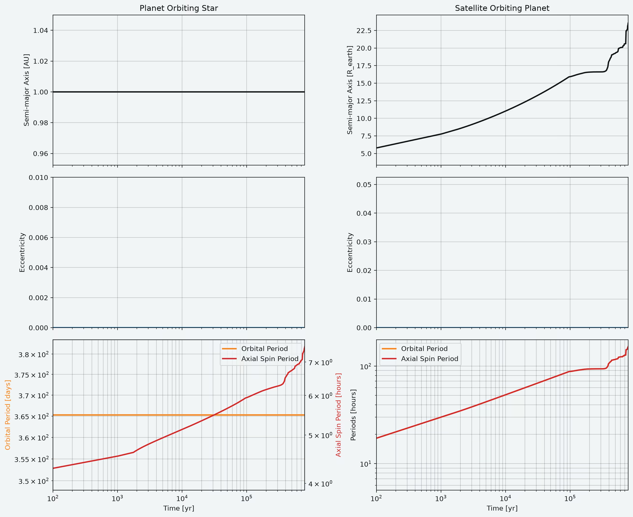
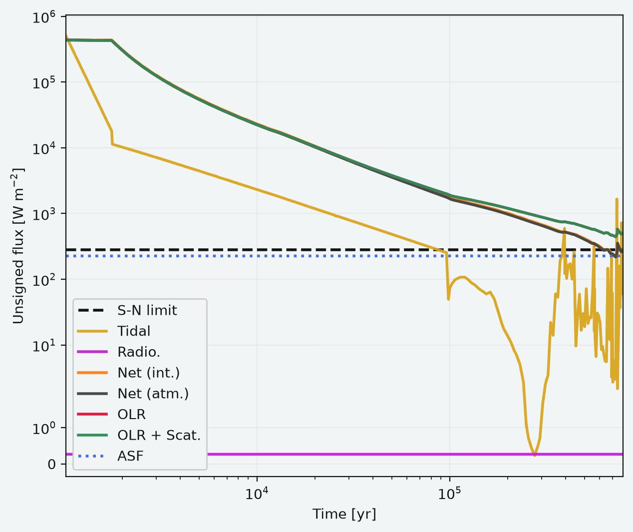
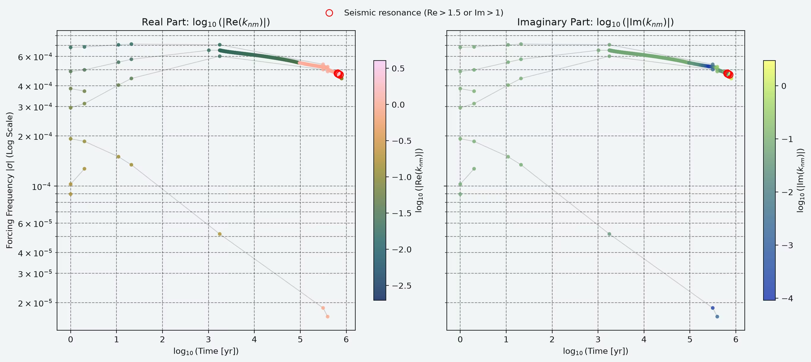
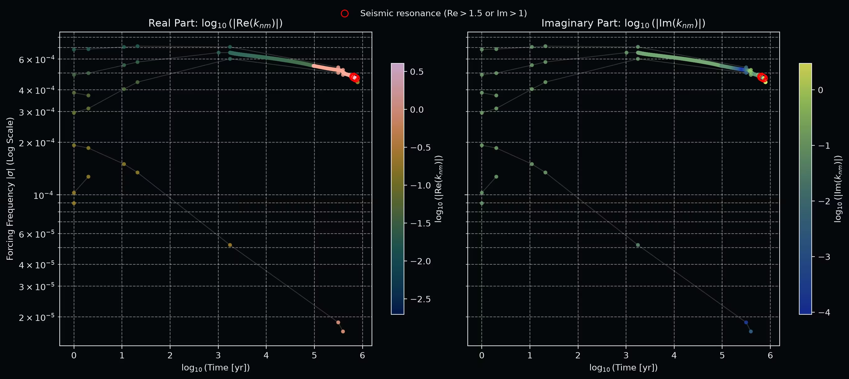
The reference run below terminates at t \(\approx\) 7.9 × 10⁵ yr once the net atmosphere-interior flux drops below the convergence threshold (status: Completed, net flux is small), with the mantle still around 20% molten (\(\Phi \approx 0.20\)) rather than fully solidified. Overall, the time steps are small enough to resolve the tidal evolution, but finer time resolution will substantially reduce the jumping behavior in the tidal heating. Ultimately, this is beyond the scope of this tutorial, as it would take substantially longer to run.

Orbital evolution — **Planet-star and satellite-planet orbital evolution.** The planet's heliocentric semi-major axis and eccentricity stay pinned at 1.00 AU and 0 (Obliqua evolves the planet-satellite pair; the star-planet orbit is not perturbed by it here), so the planet's orbital period holds at 365.2563 days while its axial (spin) period lengthens from 4.00 h to 7.52 h as the satellite despins it. The satellite's semi-major axis climbs from ~3.5 to ~23.4 Earth radii over the run, with its orbital and axial spin periods rising together from ~9.1 h to ~158.3 h (i.e. it stays tidally locked), and its eccentricity varying between 0 and 0.05.

**Global flux budget.** Tidal heating (gold) starts at ~5.0 × 10⁵ W m^-2, comparable to the net interior/atmosphere flux (orange/grey) at that time, then decreases as the satellite moves away from the planet, first dropping below the runaway-greenhouse (S–N) limit at t ≈ 8.8 × 10⁴ yr. From there it no longer decays smoothly: it reaches an absolute minimum of ~0.2 W m^-2 near 2.8 × 10⁵ yr, then fluctuates through a long series of resonance-driven bursts as the dominant tidal mode repeatedly sweeps in and out of the mantle's normal-mode resonances (see the Love-number figure below), peaking at ~1.7 × 10³ W m^-2 near 7.4 × 10⁵ yr. The mantle is still ~20% molten when the run ends at t ≈ 7.9 × 10⁵ yr, with tidal heating (~2.6 × 10² W m^-2) comparable to the net interior/atmosphere flux rather than having settled into a smoothly decaying solid-tide regime.

**Degree-2 Love number spectrum evolution (Obliqua).** The dominant, almost always populated mode is the semidiurnal (n=2, m=2, k=2) tide; its forcing frequency |σ| decreases from ~6.5 × 10^-4 to ~4.4 × 10^-4 rad s^-1 as the satellite recedes and despins the planet. Re(k₂₂) starts near 0.03 and jumps by roughly two orders of magnitude to ~1–1.3 once the forcing frequency first sweeps past a normal-mode (seismic) resonance around t ≈ 9.6 × 10⁴ yr, then fluctuates in that resonance-affected regime for most of the run. It briefly exceeds the seismic-resonance threshold (Re > 1.5, ringed in red) four times between t ≈ 6.5 × 10⁵ and 7.3 × 10⁵ yr, peaking at ~4.1 at t ≈ 7.3 × 10⁵ yr (where Im(k₂₂) also drops to its smallest value, 10^-3.0), before settling to small, occasionally negative values (~10^-1.0) by the end of the run.

Spada, F., Demarque, P., Kim, Y.C. & Sills, A., The radius discrepancy in low-mass stars: single versus binaries, The Astrophysical Journal, 776, 87, 2013. SciX. ↩