Validation: src/proteus/orbit/satellite.py¶

What this page checks¶

This page checks the planet-satellite tides of proteus.orbit.satellite: the angular momentum of the planet and its satellite, and the capture of the satellite into the evection resonance. Validation means that a test runs the code on a case with a known right answer and checks the result within a stated tolerance. If this part of the code is wrong, the spin of the planet and the orbit of the satellite evolve wrongly. Each case below says why the check exists, what it tests, how we know the right answer and why it matters. A box "Test details" ends each case.

Angular momentum of the Earth-Moon system¶

Why this check exists. The total angular momentum is the spin of the planet plus the orbit of the satellite, and the orbital term must use the satellite mass. The planet mass in its place makes the orbital term about 81 times, and the total about 66 times, too large for the Earth-Moon system, without an error message.

What it tests. ps0d is the satellite model that evolves the orbit of the satellite and the spin of the planet from angular-momentum conservation (Korenaga 2023). On its first step, ps0d computes the total angular momentum plan_sat_am with Eq. 60 of Korenaga (2023): \(L = I \Omega + M_\mathrm{sat} \sqrt{G (M_p + M_\mathrm{sat})\, a}\), with \(I\) the moment of inertia and \(\Omega\) the spin rate of the planet, \(M_p\) and \(M_\mathrm{sat}\) the masses and \(a\) the semi-major axis of the satellite. The test uses the present Earth-Moon system and compares the result with Eq. 60 evaluated in the test, without a call into the source. It also checks that the planet-mass version differs by more than 50 times, and that \(L\) lies between 1e34 and 1e35 kg m\(^2\)/s.

How we know the right answer. Eq. 60 of Korenaga (2023); its orbital term agrees with the present Earth-Moon value of Touma and Wisdom (1994), about 2.85e34 kg m\(^2\)/s (see the derivation below).

Why it matters. plan_sat_am is the total angular momentum from which the satellite model starts.

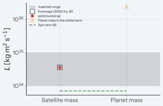
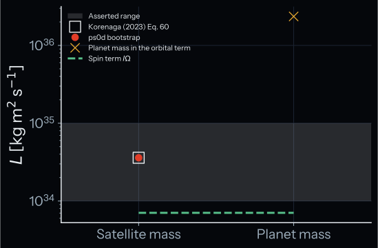
How to read the plot. The y-axis is the total angular momentum of the present Earth-Moon system, on a log scale. The filled circle is the asserted ps0d bootstrap value, and the hollow square Eq. 60 of Korenaga (2023), with the satellite mass in the orbital term. The cross is the same sum with the planet mass in the orbital term, which the test rejects. The dashed line is the spin term \(I\Omega\) alone (context). The grey band is the asserted range \(10^{34}\) to \(10^{35}\) kg m\(^2\)/s. A pass means that the circle sits in the square inside the band, and the cross far above it.

Capture into the evection resonance¶

Why this check exists. In the evection resonance the precession of the lunar orbit matches the orbital period of the Earth around the Sun, and the eccentricity of the satellite orbit grows. A wrong tidal rate or a wrong resonance term changes when the capture happens, or stops it, without an error message.

What it tests. The test runs evolve_orbit_satellite with model='ps1d_evec', the model of Correia and Valente (2022) with the evection terms of Rufu and Canup (2020), and a constant-time-lag tidal response, from the initial conditions of the Figure 3 case of Rufu and Canup (2020). The eccentricity must cross 0.1 between 2e4 and 4e4 yr.

How we know the right answer. Rufu and Canup (2020), Figure 3, captures at about 2.4e4 yr. The run recorded in the test file crossed 0.1 at 2.58e4 yr. The window from 2e4 to 4e4 yr is a regression envelope around that run, not a tolerance from the paper.

Why it matters. The capture time sets when the eccentricity of the satellite orbit starts to grow in a run with ps1d_evec.

Known limit. The test checks a time window, not the full eccentricity history.

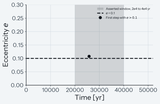
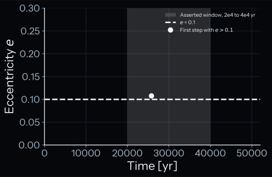
How to read the plot. The x-axis is the time and the y-axis the eccentricity \(e\). The circle is the first step of the run with \(e > 0.1\), the asserted capture into the resonance. The dashed line is \(e\) = 0.1, and the grey band the asserted window from 2e4 to 4e4 yr. The plot shows only this step, because the trajectory of the Radau solver (an implicit Runge-Kutta method of scipy.integrate.solve_ivp) changes between machines. A pass means that the circle lies in the band.

Peak eccentricity in the evection resonance¶

Why this check exists. The resonance drives the eccentricity to a peak at a given distance of the satellite. A wrong resonance term moves the peak or lowers it without an error message.

What it tests. With the same run as above, which stops at 5.2e4 yr, the highest eccentricity up to that time must reach at least 0.6, at a satellite distance \(a'\) between 10 and 13 Earth radii.

How we know the right answer. The test file gives the values of Rufu and Canup (2020), Figure 3: a peak at e of about 0.72 to 0.724 at \(a'\) of about 11.89 Earth radii, at about 5.2e4 yr. The run recorded in the test file peaked at e = 0.744 at \(a'\) = 12.33 Earth radii and 5.18e4 yr, about 4 % above the reference in \(a'\). The bounds \(e \ge 0.6\) and \(a'\) from 10 to 13 Earth radii are a regression envelope around that run, wide enough for the run-to-run changes of the Radau solver, not a tolerance from the paper.

Why it matters. The peak eccentricity and its distance set how far the resonance moves the satellite orbit in a run with ps1d_evec.

Known limit. The contraction after the peak (\(a'\) falling to about 10.2 Earth radii by 1e5 yr in the reference) is not asserted.

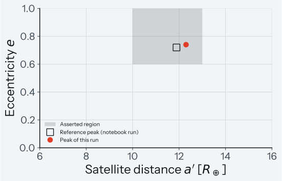
How to read the plot. The x-axis is the satellite distance \(a'\) in Earth radii \(R_\oplus\), and the y-axis the eccentricity \(e\). The circle is the asserted peak of the run, shown to 3 significant digits in \(a'\) and 2 in \(e\) against round-off between platforms. The grey region is the asserted condition: \(e \ge 0.6\) at \(a'\) between 10 and 13 \(R_\oplus\). The hollow square is the peak of Rufu and Canup (2020), Figure 3, as the test file gives it: \(e \approx 0.72\) at \(a' \approx 11.89\,R_\oplus\) (context). As in the case above, only the asserted peak is drawn. A pass means that the circle lies in the grey region.

Re-derivation note¶

The orchestrator populates plan_sat_am from

L_total = I_planet * omega_planet + M_satellite * sqrt(G (M_planet + M_sat) a_sat)

with I_planet = (2/5) M_planet R_planet^2 for a solid sphere. This is the Korenaga (2023) Eq. 60 form, equivalent to the textbook reduced-mass orbital angular momentum L_orb = mu * sqrt(G (M_pl + M_sat) a) in the M_sat << M_planet limit (where mu = M_pl M_sat / (M_pl + M_sat) -> M_sat). For the Earth-Moon system the substitution has a 1.2% relative error.

For Earth parameters, the two components evaluate to

The orbital component agrees with Touma and Wisdom (1994), who report the present-day Earth-Moon orbital angular momentum as ~2.85e34 kg m^2 / s. The total system angular momentum (spin + orbital) is ~3.6e34 kg m^2 / s, which is what plan_sat_am starts from; ps1d and ps1d_evec update it during the run. The reference-pinned test brackets the total in [1e34, 1e35] kg m^2 / s; a regression that swaps M_sat for M_planet in the orbital prefactor would land at ~2.4e36 kg m^2 / s, well outside the bracket.

Eq. 58-59: rotation and semi-major-axis rate equations¶

No test on this page checks Eq. 58-59; this section is background for the cases above.

Korenaga (2023) Eq. 58 gives the planet's spin-down rate,

dOmega/dt = -E_tide_dot / (I*Omega + G*M_pl*M_sat*I / (a*(L - I*Omega)))

where E_tide_dot is the tidal power dissipated in the planet (positive, W) and L is the conserved total angular momentum from Eq. 60. The minus sign makes the spin slow whenever tidal energy is dissipated, matching the expectation that dissipation transfers angular momentum from the planet's spin to the satellite's orbit. Eq. 59 for the semi-major axis,

da/dt = -2*I*a / (L - I*Omega) * dOmega/dt

follows directly from differentiating the Eq. 60 closure at constant L and solving for da/dt: whenever the planet's spin slows, the orbit expands, provided L > I*Omega (the prograde-satellite regime PROTEUS targets).