Parameter grid sweep

This tutorial runs an ensemble of PROTEUS simulations across a grid of parameter values using the proteus grid command. Grid runs are the standard approach for parameter studies, sensitivity analyses, and population synthesis.

It uses the all-dummy base configuration (input/dummy.toml), so every case runs in seconds without any external solver, and the whole grid finishes in a couple of minutes on a laptop. The numbers below are therefore illustrative of the workflow, not physical predictions; see the caveats at the end.

How grids work

PROTEUS generates the Cartesian product of all parameter axes. Each combination becomes an independent simulation with its own configuration file, output directory, and status tracking. The grid in this tutorial has three axes of three values each, so it produces 3 x 3 x 3 = 27 cases.

The grid configuration

A grid is described by its own TOML file, separate from a normal run config. The one used here is committed at input/tutorials/tutorial_grid.toml:

config_version = "3.0"

# Base config: each grid point starts from this all-dummy file
ref_config = "input/dummy.toml"

output  = "tutorial_grid"   # output folder inside output/
symlink = ""                # redirect output elsewhere (absolute path), or ""

use_slurm = false
max_jobs  = 8               # max concurrent cases (local)
max_days  = 1               # per-job walltime [days] (Slurm)
max_mem   = 12              # per-CPU memory [GB] (Slurm)

# Stop every case at solidification (already on in the base) or at energy
# balance, whichever comes first. A single value sets the field for all cases.
["params.stop.radeqm.enabled"]
    method = "direct"
    values = [true]

# Planet mass [M_earth]: explicit values
["planet.mass_tot"]
    method = "direct"
    values = [0.5, 1.0, 2.0]

# Orbital distance [AU]: log-spaced, close-in to moderate
["orbit.semimajoraxis"]
    method = "logspace"
    start  = 0.03
    stop   = 0.5
    count  = 3

# Hydrogen inventory [ppmw]: linearly spaced
["planet.elements.H_budget"]
    method = "linspace"
    start  = 1000
    stop   = 9000
    count  = 3

Sweep methods

Each axis declares a method that controls how its values are generated. This tutorial illustrates three of the four:

logspace and linspace take the actual endpoint values (not exponents). A single-value direct entry, like the params.stop.radeqm.enabled line above, sets a constant for every case rather than sweeping it.

Parameter paths

The table header (for example "orbit.semimajoraxis") is a dot-separated path into the PROTEUS configuration. Any field in the configuration reference can be swept.

Running

conda activate proteus
proteus grid -c input/tutorials/tutorial_grid.toml

The grid manager generates all 27 configurations, writes one per case, launches up to max_jobs at a time, and reports progress until every case has stopped.

Stop conditions

Each case runs until one of two conditions is met, whichever comes first:

• Solidification: the global melt fraction drops below phi_crit (0.01). This is enabled in the base config.
• Energy balance: the net surface flux becomes small (radiative equilibrium). The grid file turns this on for every case via the params.stop.radeqm.enabled entry.

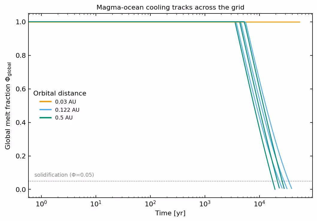
Which one triggers depends on orbital distance, as shown below.

Results

The melt-fraction histories split cleanly by orbital distance:

Each input axis controls a distinct output:

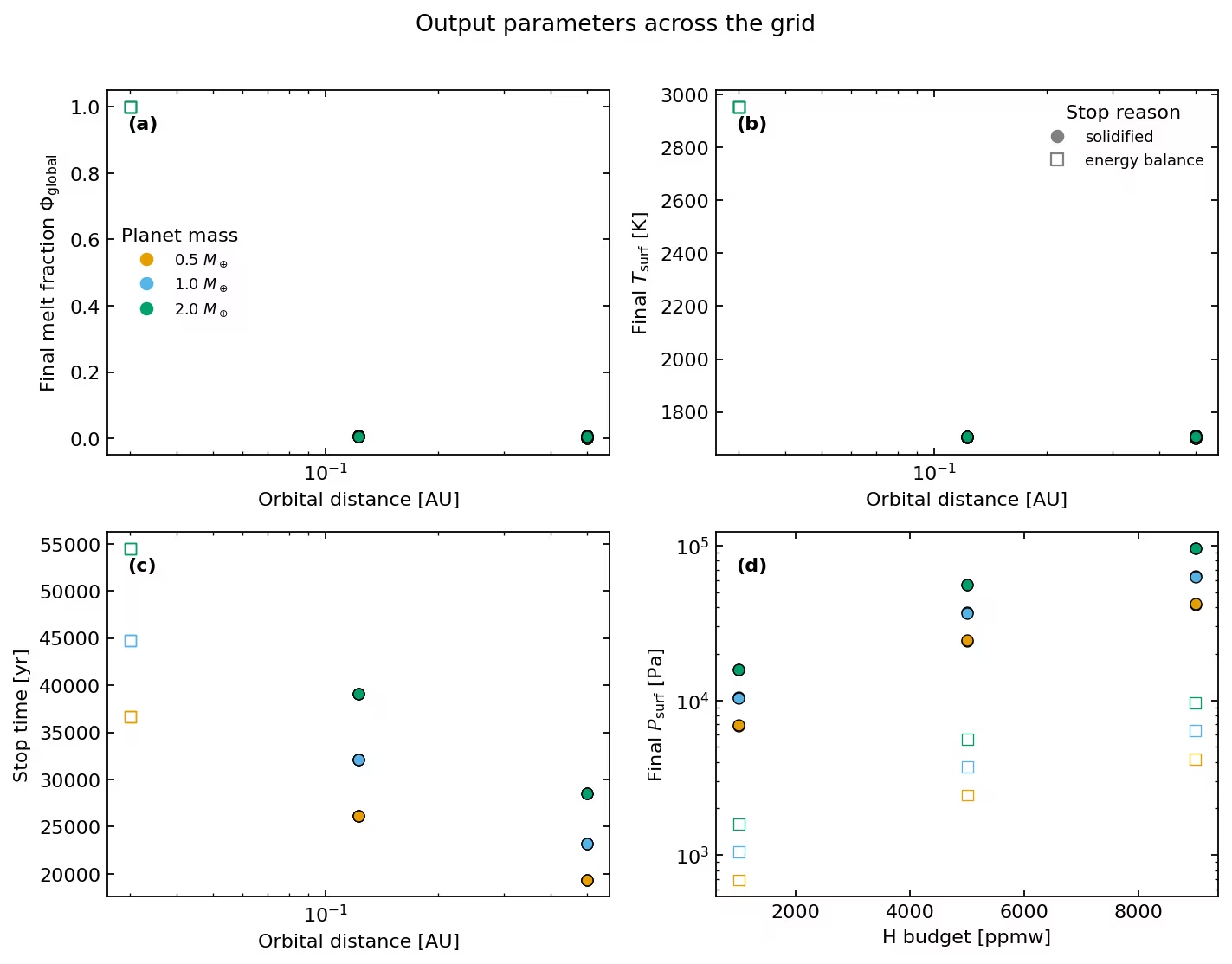
In words, for this dummy setup:

• Orbital distance sets the outcome. At 0.03 AU the instellation keeps the mantle above its liquidus, so the planet never solidifies and stops at energy balance. Farther out it solidifies. Among the solidified cases, a closer orbit gives a longer cooling time, because absorbed instellation partly offsets the surface cooling (for 1 M_earth: 32 kyr at 0.122 AU versus 23 kyr at 0.5 AU).
• Planet mass sets the timescale. A more massive planet holds more heat and takes longer to solidify (roughly 19, 23, and 28 kyr at 0.5 AU for 0.5, 1.0, and 2.0 M_earth).
• Hydrogen budget sets the surface pressure. More hydrogen outgasses a thicker atmosphere (surface pressure scales with H_budget), but in this dummy setup it does not change the cooling rate or the thermal endpoint.

Monitoring progress

proteus grid-summarise -o output/tutorial_grid

This reports how many cases are running, completed, or failed. Filter by status:

proteus grid-summarise -o output/tutorial_grid -s completed
proteus grid-summarise -o output/tutorial_grid -s error

Results files

Each case writes to output/tutorial_grid/case_NNNNNN/. The grid directory also holds manager.log, ref_config.toml (the base config), copy.grid.toml (the grid definition), and cfgs/ (the per-case configs), so the ensemble is reproducible from its output folder alone.

Packing results

proteus grid-pack -o output/tutorial_grid

This writes output/tutorial_grid/pack.zip with the helpfile, status, and log for each case (and plots, if present).

Analysis

Load every case, recover its swept inputs from the resolved per-case config, and tabulate the final state:

import pandas as pd
import toml
from pathlib import Path

grid = Path('output/tutorial_grid')
rows = []
for case in sorted(grid.glob('case_*')):
    code = int((case / 'status').read_text().splitlines()[0])
    if not (10 <= code <= 19):        # keep only completed cases
        continue
    cfg = toml.load(case / 'init_coupler.toml')
    df = pd.read_csv(case / 'runtime_helpfile.csv', sep='\t')
    last = df.iloc[-1]
    rows.append({
        'mass': cfg['planet']['mass_tot'],
        'sma': cfg['orbit']['semimajoraxis'],
        'H_ppmw': cfg['planet']['elements']['H_budget'],
        't_stop': last['Time'],
        'Phi_final': last['Phi_global'],
        'P_surf': last['P_surf'],
    })
summary = pd.DataFrame(rows)
print(summary)

Slurm cluster execution

For large grids on HPC clusters, set use_slurm = true and raise the limits:

use_slurm = true
max_jobs  = 500      # max concurrent Slurm array tasks
max_days  = 2        # walltime per case [days]
max_mem   = 12       # memory per CPU [GB]

The grid manager then writes a Slurm job-array script and prints the sbatch command to submit it. Each case runs as an independent array task. See the cluster guides (Habrok, Snellius).

Caveats: this is the dummy model

The all-dummy base makes the grid fast but parameterises the physics. In particular: the grey atmosphere uses a fixed greenhouse factor, so the hydrogen budget does not feed back on the cooling rate; the surface temperature is set equal to the mantle temperature; and the solidified surface temperature is pinned to the mantle solidus by construction. The 0.03 AU axis endpoint is an extreme close-in orbit, chosen so the grid brackets the molten-to-solidified transition. With the real modules (AGNI, SPIDER or Aragog, CALLIOPE) the orbital and compositional dependence is stronger, because the outgoing radiation then depends on atmospheric pressure and composition. Treat the numbers here as a demonstration of the grid workflow.

Exercises

1. Add an fO\(_2\) axis with arange: sweep outgas.fO2_shift_IW from \(-2\) to \(+4\) in steps of 2, to exercise the fourth sweep method.
2. Widen the orbital axis (for example logspace 0.02 to 1.0, count 5) and see where the molten-to-solidified transition lands.
3. Swap the base for a real-physics config (change ref_config to your Earth analogue config) and rerun a smaller grid.

See also: Parameter grids how-to | Configuration file | Earth analogue tutorial