Quick start: all-dummy run
This tutorial runs PROTEUS with all modules set to "dummy" backends. No external solvers (AGNI, SPIDER, SOCRATES) are needed; the run completes in under a minute and exercises the full coupling architecture. Use this to verify your installation and understand the code flow before moving to production runs.
Prerequisites
- PROTEUS installed (
pip install -e ".[develop]") FWL_DATAenvironment variable set
No external solvers, spectral files, or EOS data are required.
The configuration file
PROTEUS ships with an all-dummy config at input/dummy.toml. The key
settings are:
- Planet: 1 M\(_\oplus\), starting fully molten (T\(_\mathrm{magma}\) = 4000 K, \(\Phi\) = 1). Volatile budget of 10,000 ppmw H, 1000 ppmw C, 500 ppmw N, 500 ppmw S.
- Star: fixed solar luminosity (no evolution)
- Orbit: 0.5 AU, weak tidal heating
- Interior structure: Noack & Lasbleis (2020) 1 analytical scaling laws
- Interior energetics: heat-capacity integrator with prescribed solidus (1700 K) and liquidus (2700 K)
- Outgassing: melt-fraction-dependent partitioning; 10% of volatiles are always in the atmosphere (finite solubility floor), with the atmospheric fraction increasing as the mantle solidifies
- Atmosphere: grey-body opacity (\(\gamma\) = 0.5)
- Escape: disabled (rate = 0), so the run reaches solidification
- Chemistry: parameterised vertical profiles (offline)
The simulation terminates when the global melt fraction drops below the solidification threshold.
Running the simulation
conda activate proteus
proteus start --offline -c input/dummy.toml
The --offline flag skips data downloads. The run should complete in
under 30 seconds.
Expected output
The run creates a directory inside output/ named with a timestamp.
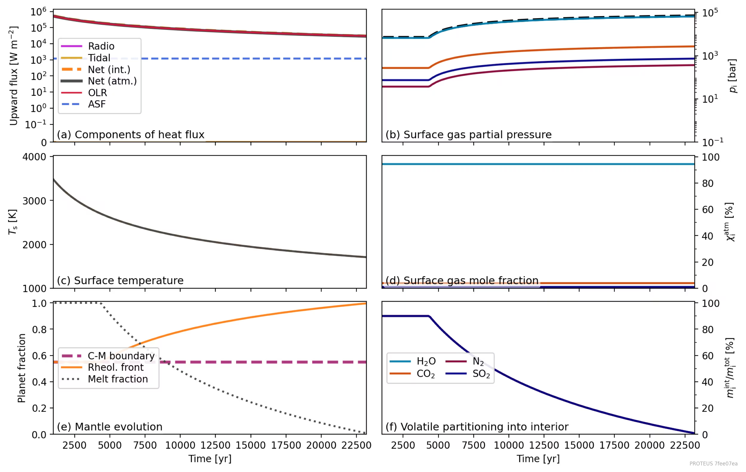
Check plots/plot_global_lin.png for a multi-panel overview. Your
output should look similar to this:
To regenerate these plots from your own output:
proteus plot -c input/dummy.toml all
Understanding the helpfile
Open runtime_helpfile.csv in the output directory to see the full time
series. Key columns:
| Column | Units | What to expect |
|---|---|---|
Time |
yr | Stays at 0 for the first 3 iterations (init stage), then advances to ~23,000 yr |
T_magma |
K | Decreases monotonically from 4000 to ~1700 |
Phi_global |
1 | Drops from 1.0 to ~0.01, triggering the solidification stop |
P_surf |
bar | Increases from ~7,000 to ~70,000 as volatiles outgas |
F_atm |
W m\(^{-2}\) | Outgoing longwave radiation; decreases as the surface cools |
F_int |
W m\(^{-2}\) | Interior heat flux; tracks F_atm in the dummy coupling |
M_planet |
kg | Constant throughout (mass conservation) |
What to look for
-
Cooling and solidification:
T_magmadecreases smoothly from 4000 K. When it crosses the solidus (~1700 K),Phi_globalapproaches zero and the run terminates with "Planet solidified!!". -
Outgassing: as the melt fraction drops, volatiles transfer from the interior to the atmosphere.
P_surfincreases and the dissolved fraction in panel (f) decreases. This is the core coupling feedback that the production modules (CALLIOPE, Aragog) compute with full thermodynamics. -
Energy balance: the OLR (red line in panel a) and interior flux (orange dashed) track each other because the dummy atmosphere directly couples
F_int = F_atm. The absorbed stellar flux (blue dashed) is constant because the star is fixed. -
Mass conservation:
M_planetshould remain constant within rounding. No atmospheric escape occurs in this configuration.
Next steps
- Vary the greenhouse effect: increase
atmos_clim.dummy.gammatoward 1.0 to slow cooling (more opaque atmosphere traps more heat) or decrease it toward 0 for faster cooling (more transparent) - Enable escape: set
escape.dummy.rate = 1e4andparams.stop.escape.enabled = trueto see atmospheric mass loss - Change volatile inventory: increase
H_budgetto 50,000 ppmw for a thicker steam atmosphere, or decrease it to 1,000 ppmw for faster solidification - Move to production modules: the Earth analogue tutorial uses Aragog, Zalmoxis, CALLIOPE, and AGNI for a quantitatively meaningful simulation
See also: Model description | Dummy modules | Coupling loop | Configuration reference | Output format
-
Noack, L. & Lasbleis, M., Parameterisations of interior properties of rocky planets, Astronomy & Astrophysics, 638, A129, 2020. SciX. ↩