Solar System CHILI intercomparison¶

The CHILI (Coupled atmospHere Interior modeL Intercomparison) project is a community benchmark that fixes shared initial and boundary conditions for magma ocean evolution codes ¹. Its first intercomparison applies that protocol to the inner Solar System, modelling the primordial magma oceans of Earth and Venus.

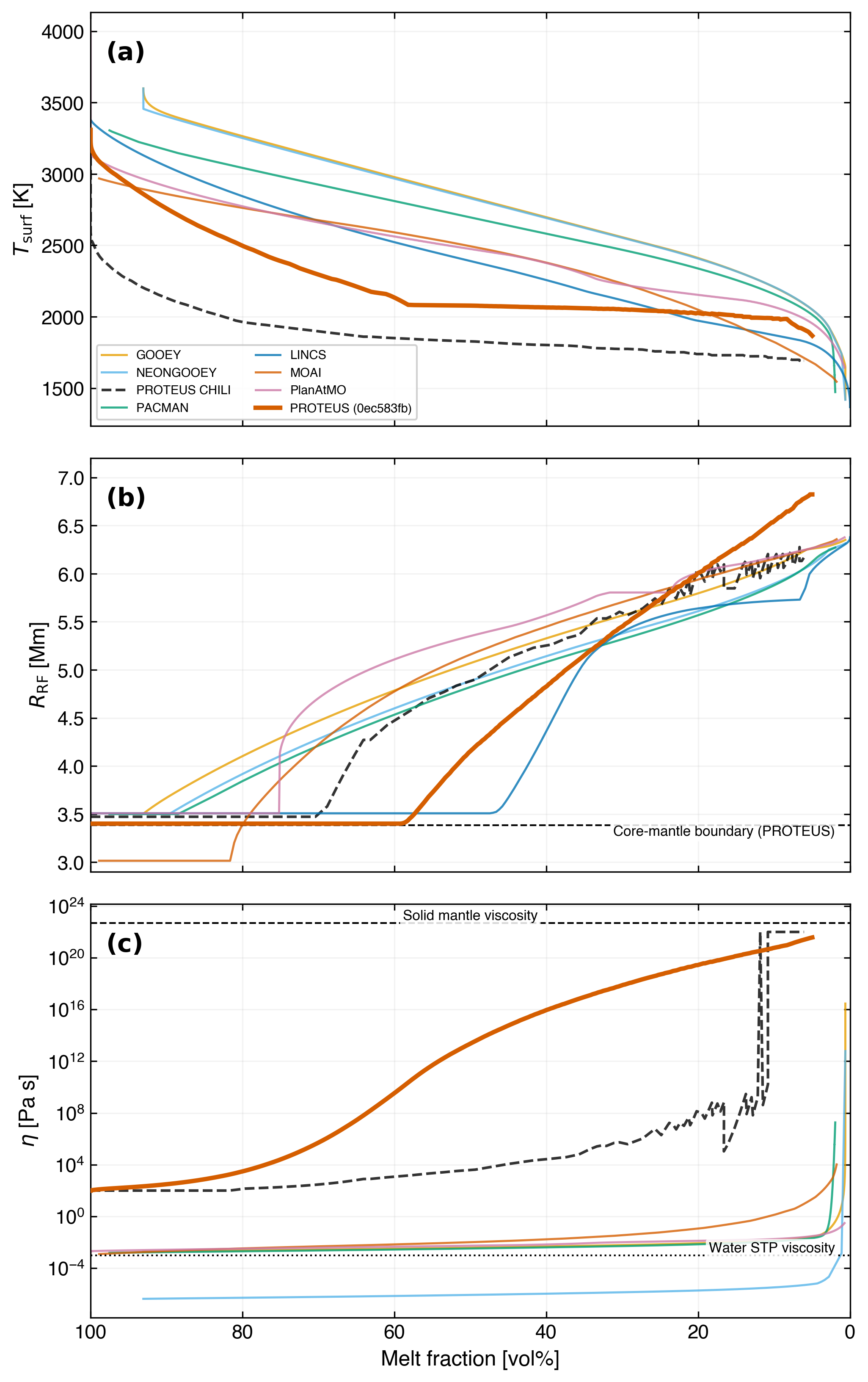
This tutorial reproduces the Solar System CHILI test suite with PROTEUS and compares the result against six other coupled atmosphere-interior models: GOOEY, NEONGOOEY, PACMAN, LINCS, MOAI, and PlanAtMO. The figures below reproduce the intercomparison plots: each one overlays the current PROTEUS run on the results submitted by every participating model. Those submitted results, and the figure layouts they follow, are drawn from the Solar System CHILI intercomparison paper (Nicholls et al. 2026) ².

Overview¶

The CHILI intercomparison defines three solar system test cases:

All cases start fully molten at 50 Myr stellar age (TRAPPIST-1 α at 1 Gyr) with BSE composition, fO\(_2\) = IW+4, and Bond albedo = 0.1. The protocol asks for a run until solidification, or for at most 1 Gyr, for the Earth and Venus cases ¹. Every run on this page stops when the melt fraction falls to 5% by mass (params.stop.solid.phi_crit = 0.05); the other stop settings below are the ones each run used, from the init_coupler.toml in its output folder. The Nominal Earth, TRAPPIST-1 e and low-H and mid-H Earth grid runs had the energy-balance, escape and wall-clock stops on, a time limit of 5 Gyr (7.55 Gyr for TRAPPIST-1 e) and a limit of 9000 iterations. The Nominal Venus run, the three high-H Earth grid runs, and the TRAPPIST-1 α and b runs had these stops off (params.stop.radeqm.enabled, params.stop.escape.enabled and params.stop.clock.enabled set to false), a 1 Gyr model time limit (params.stop.time.maximum = 1e9), and a limit of 1,000,000 iterations (params.stop.iters.maximum). The repository configs in input/chili/intercomp/ carry this second set of settings for every case. In all runs the iteration limit and the stall stop stay on; the stall stop ends a run as an error after 150 consecutive iterations without a converged atmosphere solve (params.stop.stall.maximum). The runs submitted to the intercomparison stop at 5% melt as well, with the energy-balance and escape stops off. Melt fractions of the current PROTEUS runs are by mass on this page unless stated otherwise, and the figures show the melt fractions of the intercomparison data by volume.

Prerequisites¶

• Full PROTEUS installation (see Installation)
• AGNI, SOCRATES, and all reference data
• Spectral files downloaded (proteus get spectral -n Dayspring -b 48)
• Solar spectrum downloaded (proteus get stellar)
• Interior data downloaded, including the PALEOS EOS tables (proteus get interiordata --config-path input/chili/intercomp/earth.toml)
• git (to clone the CHILI comparison data)
• The runs on this page that reached 5% melt took about 2.7 hours to about 5.5 days of wall time (Nominal Venus). Of the five runs stopped before reaching 5% melt, the three high-H Earth grid runs and the TRAPPIST-1 b run used 6.95 to 7.21 days, and the TRAPPIST-1 α run 0.91 days. These are elapsed wall-clock times. In the logs of nine of the runs, two consecutive timestamps lie 3 to 12 hours apart (seven of these intervals start on 12 October between 09:29 and 10:41), and the elapsed times include these intervals. A run that stays partly molten takes steps of at most 4000 yr (params.dt.mushy_maximum), so at least 250,000 steps to reach 1 Gyr.

The commands below run with --offline, which skips the automatic reference-data check, so all data must be on disk beforehand. Drop the flag to let the first run download missing data instead.

Step 1: Run the nominal cases¶

conda activate proteus

# Earth (see also the Earth analogue tutorial for detailed analysis)
mkdir -p output/chili_earth
nohup proteus start --offline -c input/chili/intercomp/earth.toml \
    > /tmp/proteus_earth_launch.log 2>&1 & disown

# Venus
mkdir -p output/chili_venus
nohup proteus start --offline -c input/chili/intercomp/venus.toml \
    > /tmp/proteus_venus_launch.log 2>&1 & disown

Monitor progress with tail -f output/chili_earth/proteus_00.log (the log appears once PROTEUS has initialized).

Step 2: Download comparison data¶

Clone the CHILI repository to access results from the other codes:

git clone https://github.com/projectcuisines/chili.git /tmp/chili

Step 3: Generate comparison plots¶

# Nominal cases only
python tools/plot_chili_comparison.py \
    --proteus-earth output/chili_earth/ \
    --proteus-venus output/chili_venus/ \
    --chili-repo /tmp/chili \
    --output output_files/chili_plots/

# With the Earth volatile grid (after running the grid cases)
python tools/plot_chili_comparison.py \
    --proteus-earth output/chili_earth/ \
    --proteus-venus output/chili_venus/ \
    --grid-dir output/ \
    --chili-repo /tmp/chili \
    --output output_files/chili_plots/

tools/plot_chili_comparison.py writes every figure on this page to the --output directory (here output_files/chili_plots/, which is gitignored) as both PDF (vector) and PNG. The colours follow the CHILI analysis code: six of the seven models are in Paul Tol's bright scheme, and PROTEUS has the orange of that code. The gases are in the PROTEUS gas colours; H₂S, O₂ and the elements H and C of Figure 4 take the colours of the CHILI analysis code. The script draws under the active matplotlib style, and --style light or --style dark applies the PROTEUS plot style of the proteus-mpl package for a direct call. The figures of this page come from tools/make_docs_figures.py, which calls the script once per figure and style. The script is version-general:

• Run from the command line, it clones the CHILI comparison data automatically if --chili-repo does not already point to a checkout, so Step 2 is optional. tools/make_docs_figures.py needs an existing checkout, given with its own --chili-repo.
• It reads the git commit of the runs from their logs (proteus_00.log of the Earth run, the Venus run and the grid runs) and puts it in the label of the current PROTEUS curves, so every figure records the code version that produced the runs. Runs of different commits give a label with each commit, separated by /. A run folder without a log, or a log without a commit, adds unknown to the label.
• --proteus-earth and --proteus-venus are optional; omit either to plot the intercomparison models alone.

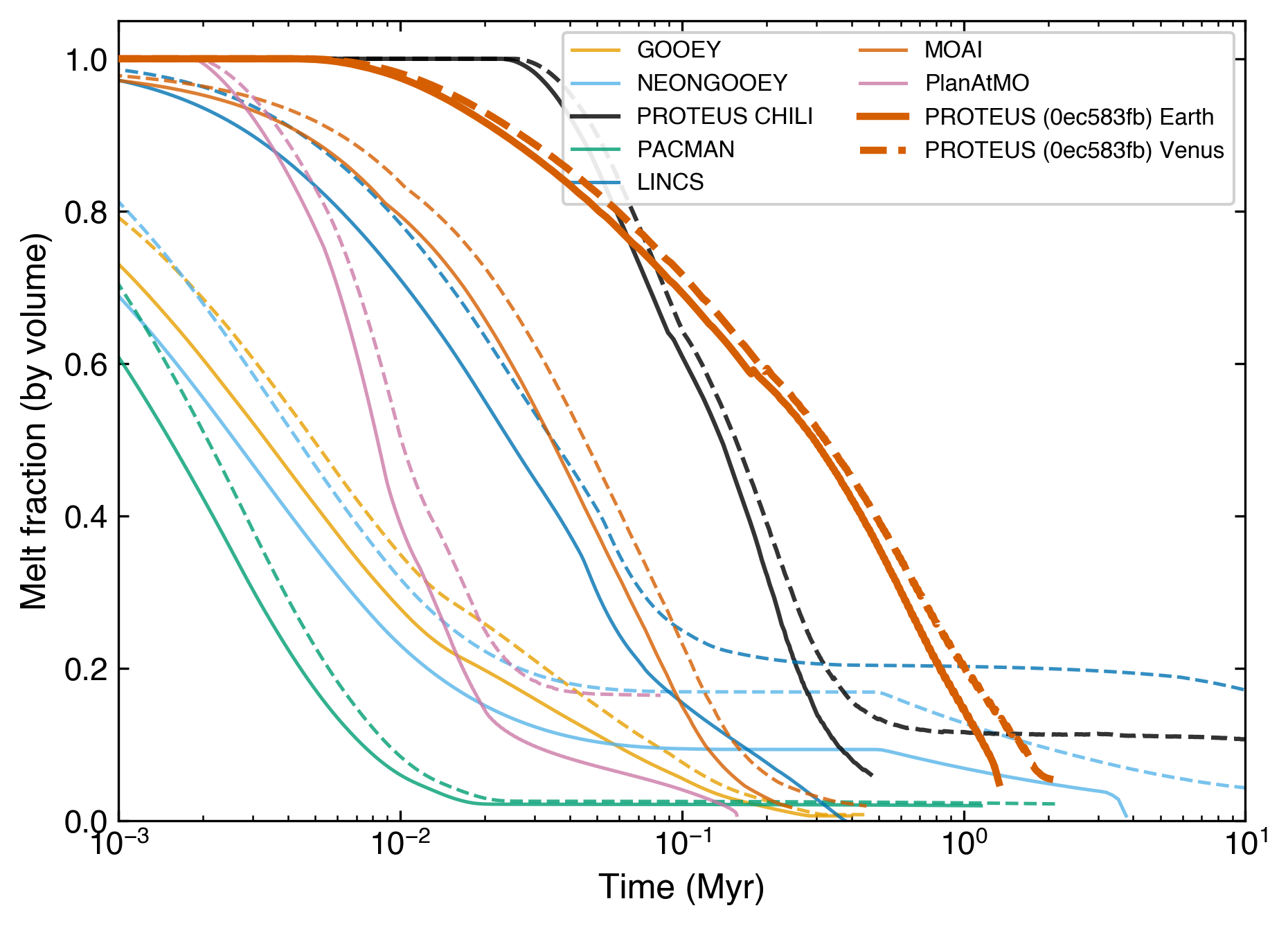
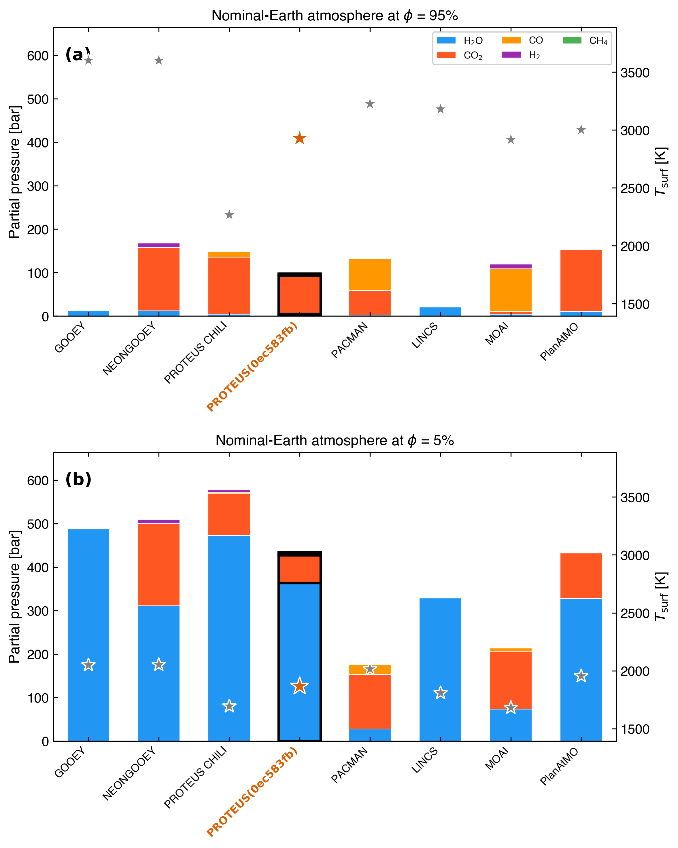
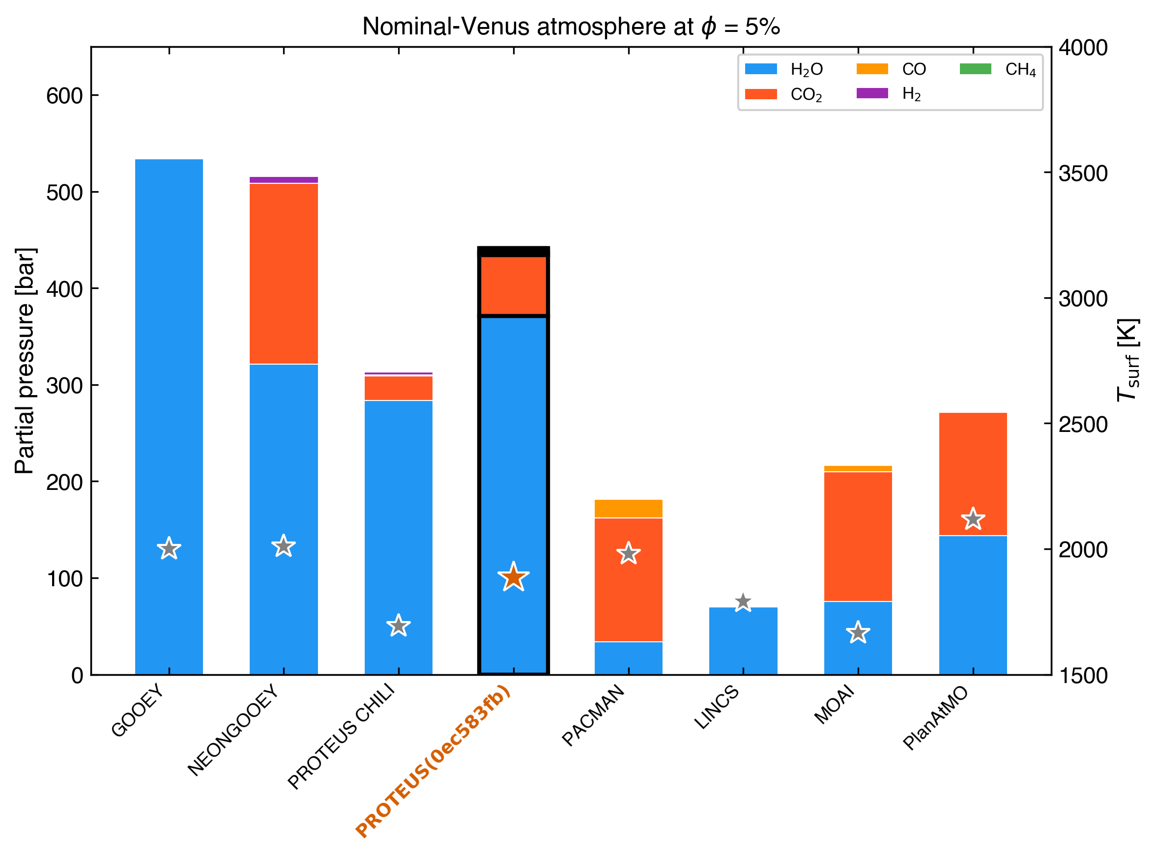
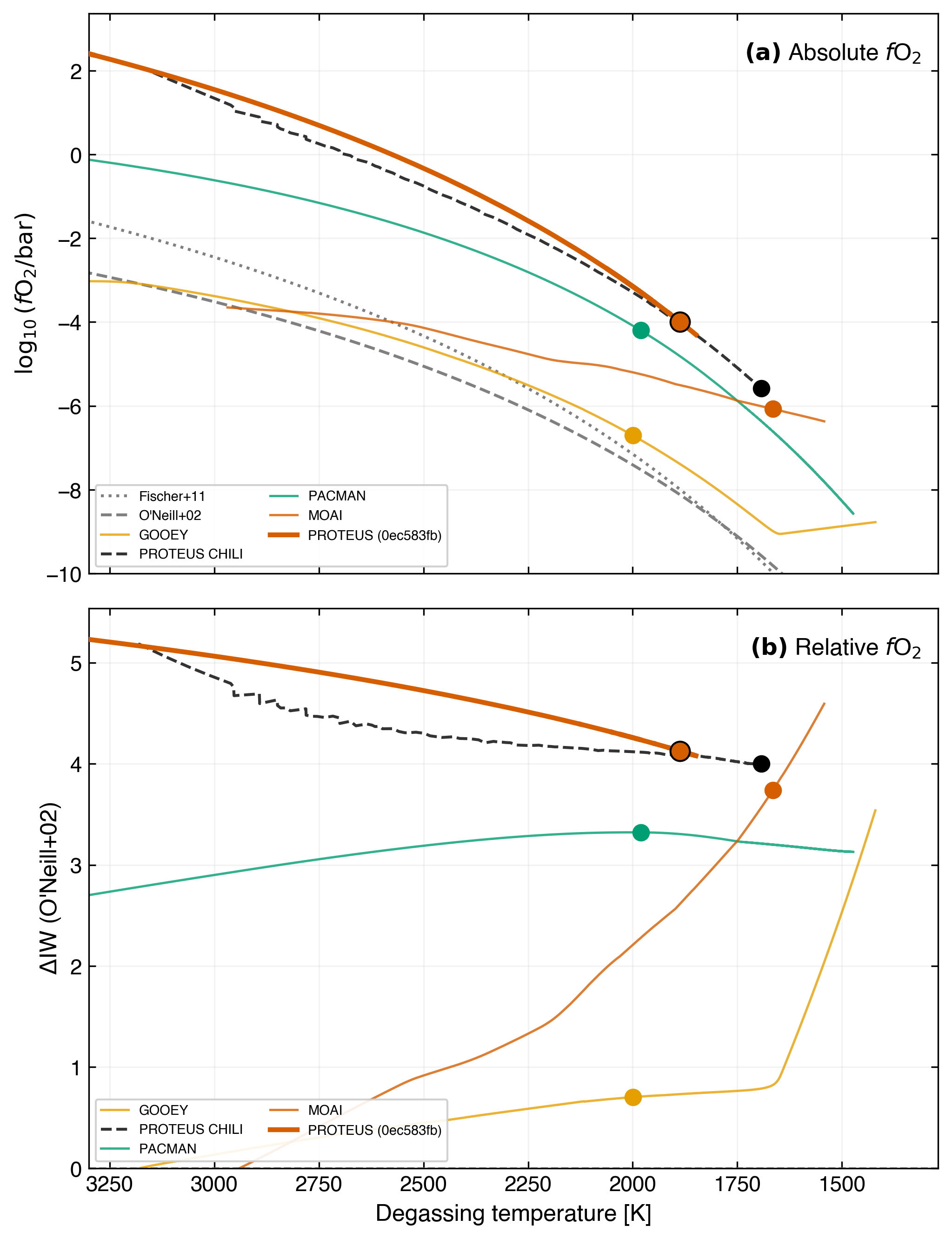
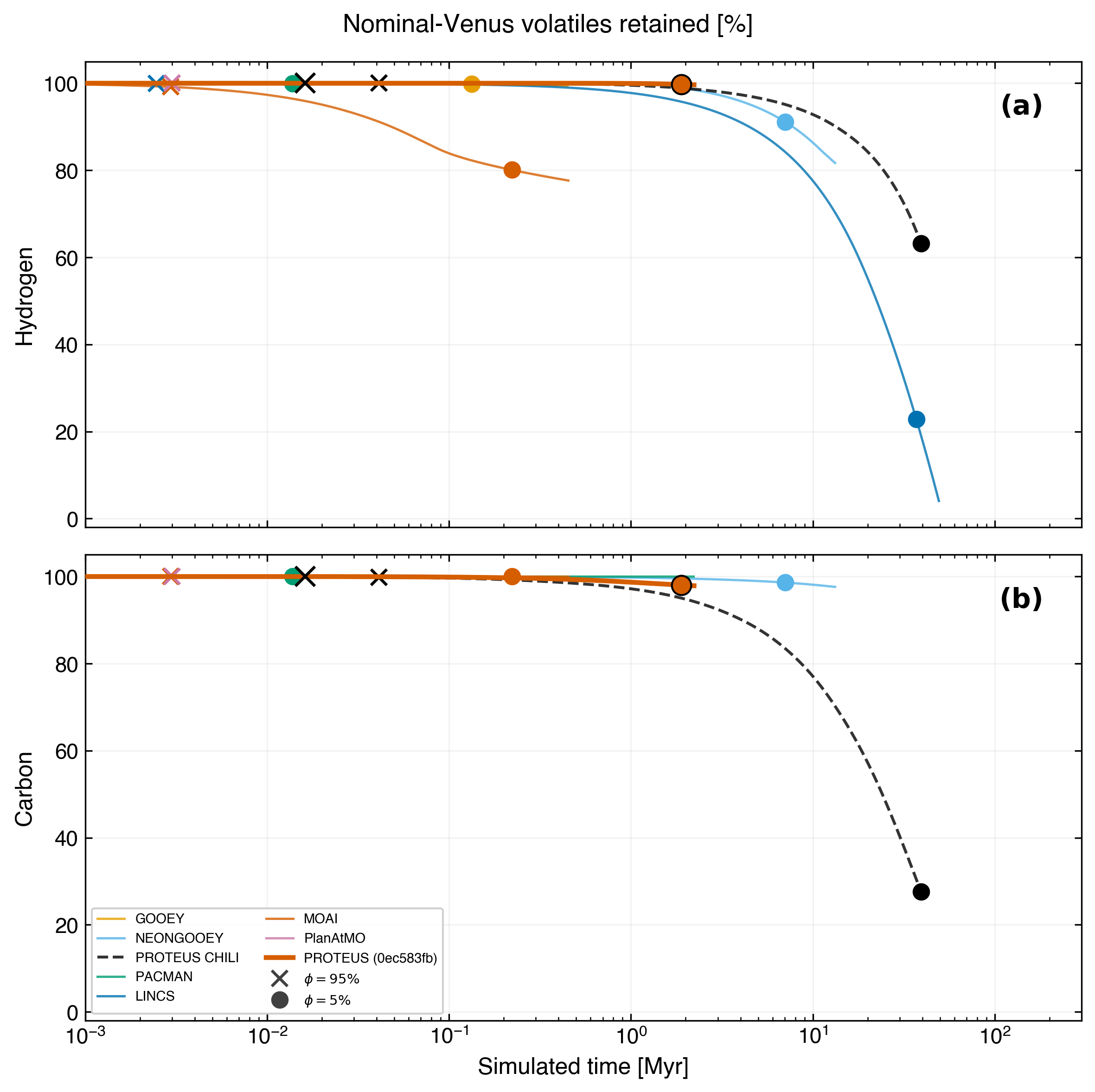
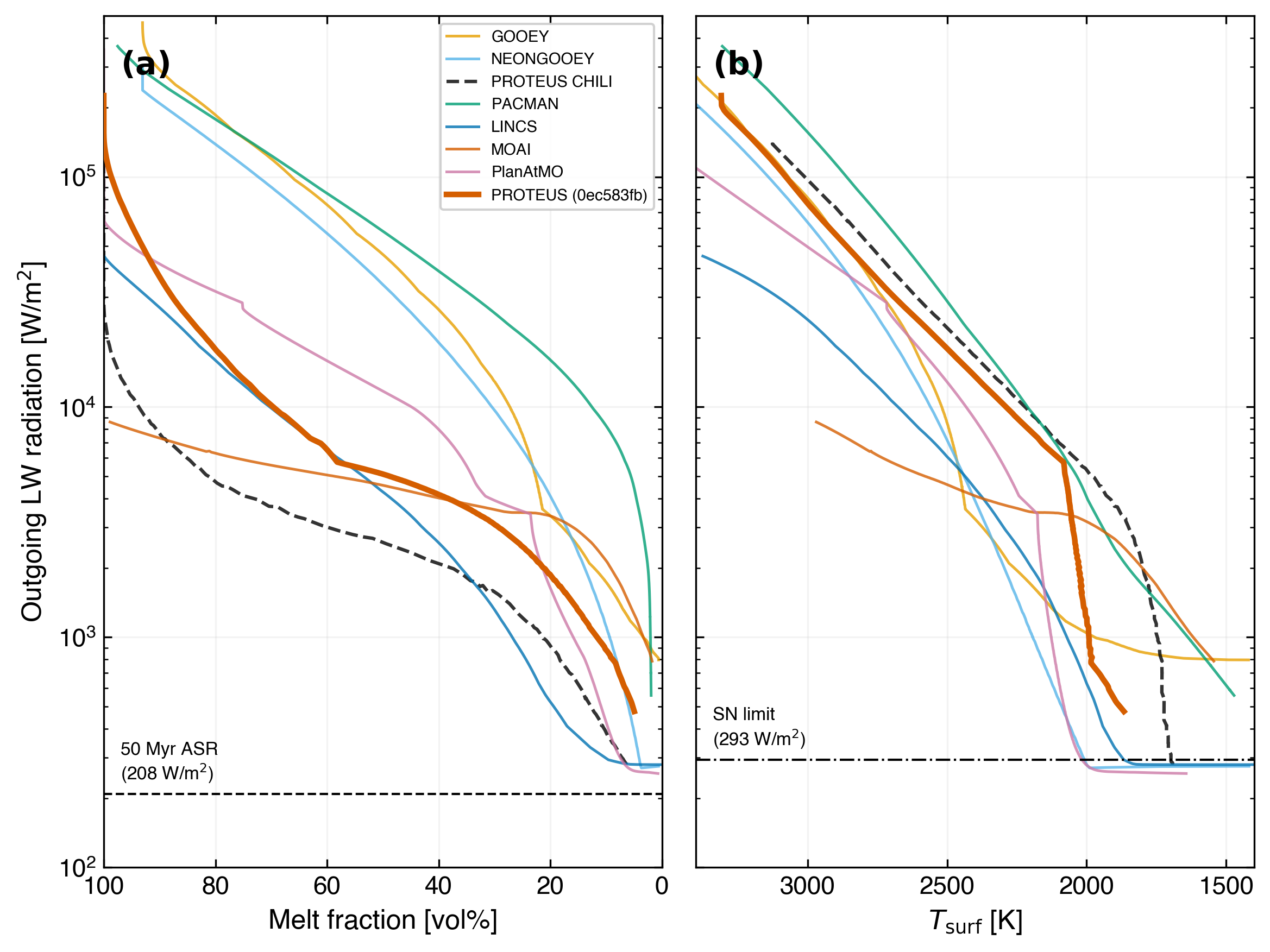
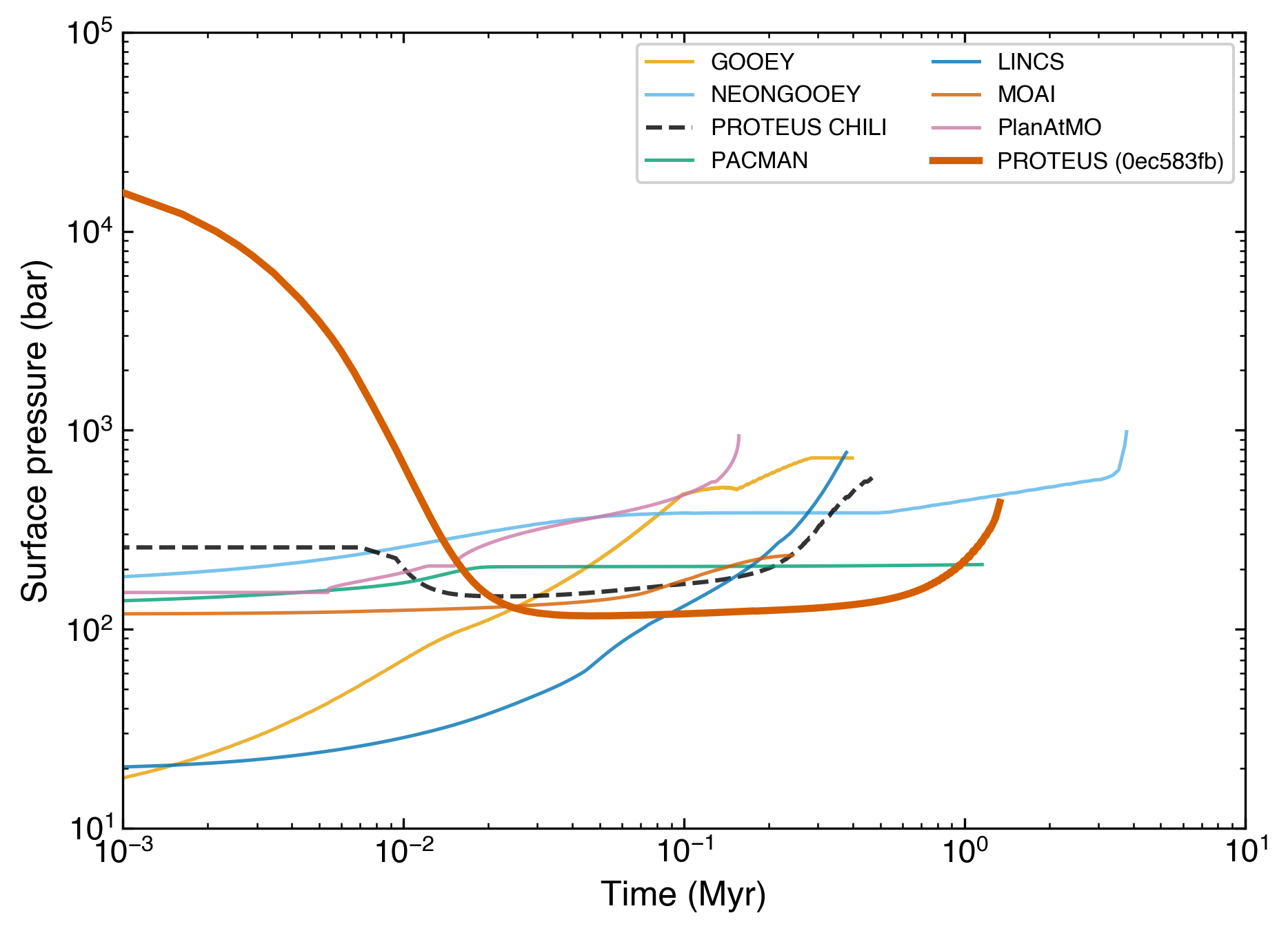
Up to two PROTEUS results appear on each plot. The results submitted to the intercomparison (Nicholls et al. 2026) are labelled "PROTEUS CHILI". In the figures with curves they are a thin orange line, dashed except in Figure 1, where the line style tells the planets apart; in Figures 3, 4 and 5 they are a bar. The current run is drawn in the same orange with thick lines and edged markers, or as a bar with an outline and a bold label, and carries the commit of the runs in its label. Running the command on the output of a future PROTEUS version draws every figure with the commit of those runs, so the comparison stays reproducible without editing the script.

Melt fraction evolution¶

Solidification milestones¶

Atmospheric composition¶

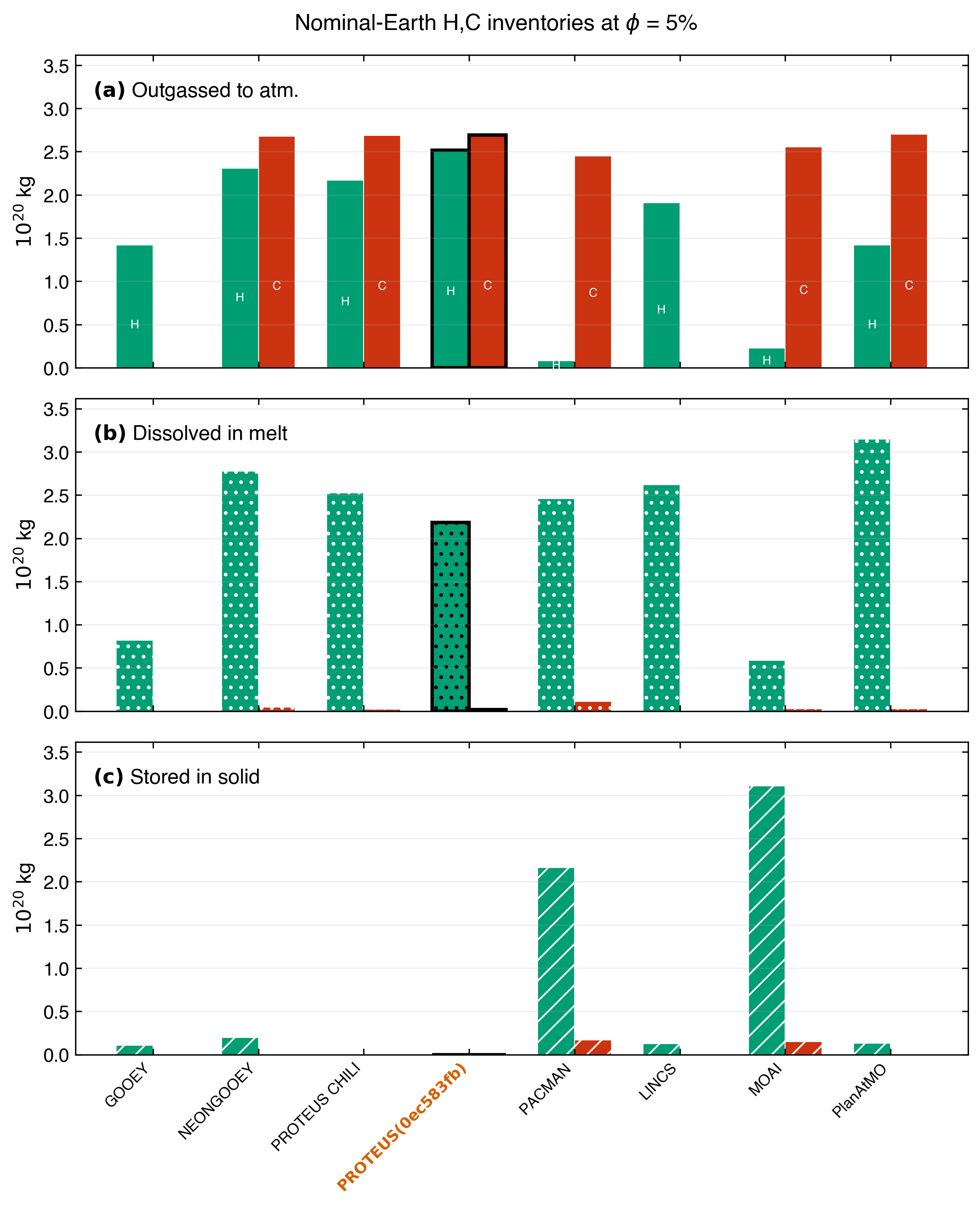
H and C mass budgets¶

Venus atmospheric composition¶

Oxygen fugacity¶

Volatile retention¶

Outgoing longwave radiation¶

Geodynamics diagnostics¶

Surface pressure evolution¶

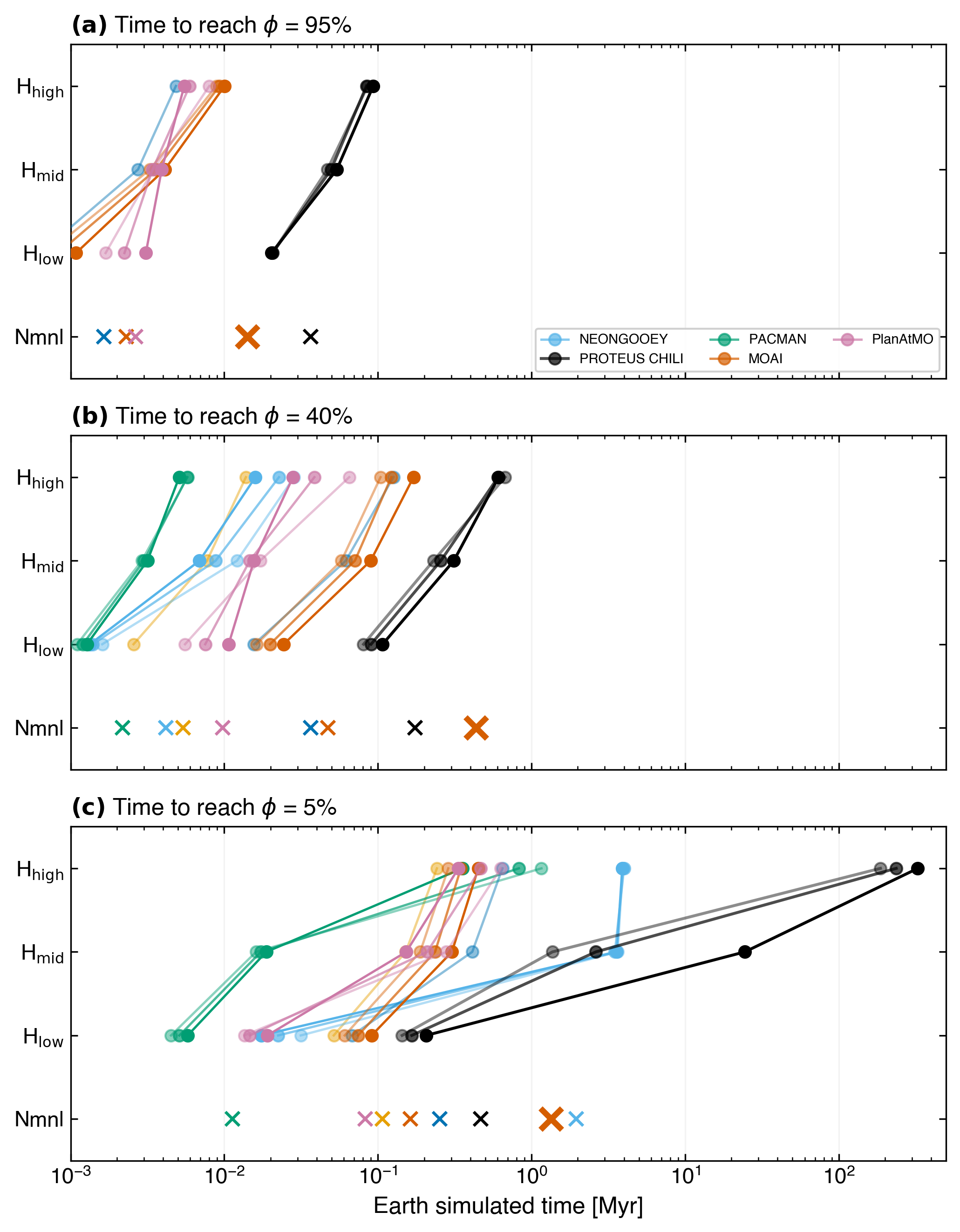
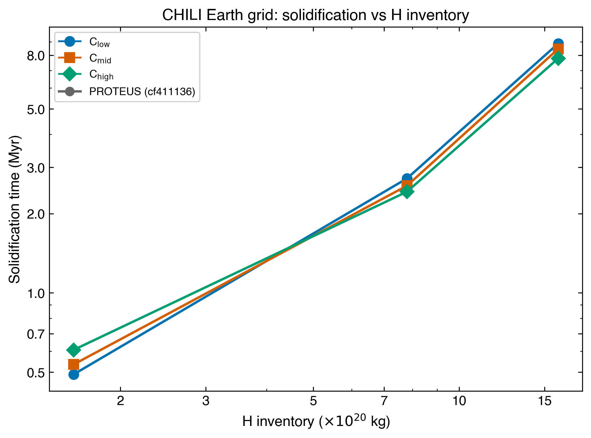
Earth volatile grid¶

The CHILI Earth grid varies H and C inventories across 9 combinations to explore how volatile budgets control solidification timescale:

Grid configs are in input/tutorials/chili_grid/. Run all 9 cases:

for cfg in input/tutorials/chili_grid/*.toml; do
    name=$(basename "$cfg" .toml)
    outdir="output/chili_grid_earth_${name#earth_}"
    mkdir -p "$outdir"
    nohup proteus start --offline -c "$cfg" \
        > "/tmp/proteus_grid_${name}.log" 2>&1 & disown
done

Check status of running grid cases:

for d in output/chili_grid_earth_*/; do
    printf "%-40s %s\n" "$(basename $d)" "$(cat $d/status 2>/dev/null || echo 'not started')"
done

Grid results¶

Time at which each grid run shown here first reaches a melt fraction of 5% by mass:

The three high-H runs were stopped before reaching 5% melt, at 60.9 to 78.2 Myr; the table gives their melt fraction there.

The hydrogen inventory is the primary control on the solidification time. From 1 to 5 EO the time to 5% melt rises by a factor of 5.3 to 6.8. At 10 EO no run reached 5% melt before being stopped at 60.9 to 78.2 Myr. The carbon effect is secondary and changes sign. At low H, more carbon slows the cooling (0.81 to 0.92 Myr): at a melt fraction of 30% the OLR falls from 5525 to 4235 W m\(^{-2}\) from low to high C. At mid H the order reverses (5.55 to 4.89 Myr): at a melt fraction of 30% the OLR rises from 1115 to 1323 W m\(^{-2}\) from low to high C. The high-H runs follow the order of the mid-H runs: at the common time of 60.9 Myr the melt fraction is 5.9%, 6.2% and 6.6% for C\(_\mathrm{high}\), C\(_\mathrm{mid}\) and C\(_\mathrm{low}\), with higher carbon corresponding to lower melt fraction.

Current PROTEUS configuration vs the CHILI submission¶

The figures show up to two PROTEUS results, and the gap between them is itself informative because the two come from different model configurations. The protocol fixes the inputs that both share: a bulk-silicate-Earth composition, oxygen fugacity at IW+4, a Bond albedo of 0.1, and a 50 Myr stellar age ¹. The two differ in the interior modules and in the limits of the stop rule: the submitted configs stop after 4.517 Gyr (6.6 and 7.55 Gyr for the TRAPPIST-1 cases) or 9000 iterations. All current runs shown here stop at 5% melt. Besides that, the Nominal Earth, TRAPPIST-1 e and low-H and mid-H grid runs stop after 5 Gyr (7.55 Gyr for TRAPPIST-1 e) or 9000 iterations with the energy-balance, escape and wall-clock stops on, while the Nominal Venus, high-H grid and TRAPPIST-1 α and b runs ran with these stops off, a 1 Gyr limit and 1,000,000 iterations, the settings the repository configs carry.

The PROTEUS results submitted to the intercomparison were computed with an earlier version of PROTEUS, not the configuration documented here. The config file of the submitted Venus run is archived with the comparison data (intercomparison/inputs/proteus/evolution-proteus-venus-config.in). It selects SPIDER for the interior thermal evolution (interior.module = "spider") and the structure calculation built into that version (struct.module = "self"), together with AGNI, CALLIOPE, ZEPHYRUS and MORS. It names VULCAN for the atmospheric chemistry, set to run only on request (atmos_chem.when = "manually" in that version, atmos_chem.mode = "none" now). Its energy balance stop criterion is switched off. See Lichtenberg et al. (2026) ¹ and Nicholls et al. (2026) ² for further details.

The configuration documented on this page uses Aragog for the interior thermal evolution and Zalmoxis for the interior structure, with AGNI for the atmosphere, CALLIOPE for the outgassing, ZEPHYRUS for the escape and MORS for the star; the three TRAPPIST-1 configs run without an escape module (escape.module = "none"). Aragog is the Python reimplementation of SPIDER and integrates the same specific-entropy equation for a two-phase, partially molten mantle with a mixing-length convective closure. Zalmoxis solves the layered interior (mass, radius, density profile, and core-mantle-boundary radius) directly and supplies the pressure-entropy equation-of-state tables that Aragog reads.

The configuration also departs from the protocol table in two inputs. The protocol fixes a planet radius (1 R\(_\oplus\) for Earth, 0.95 R\(_\oplus\) for Venus) and a core radius fraction of 0.55 ¹. Here Zalmoxis solves the structure from a core mass fraction of 0.325, which gives a radius of 7.03 Mm (1.10 R\(_\oplus\)) for Earth and 6.63 Mm (1.04 R\(_\oplus\)) for Venus, each with a core radius fraction of 0.49. The protocol sets the stellar irradiance to 920 W m\(^{-2}\) for Earth and 1760 W m\(^{-2}\) for Venus; the runs take it from the stellar evolution model, 1005 and 1923 W m\(^{-2}\) at their start.

The Nominal Venus case¶

The Nominal Venus run reached the 5% melt threshold at 86.8 Myr, where its melt fraction is 0.050 by mass (0.061 by volume). The run submitted to the intercomparison ends at 39 Myr with a melt fraction of 0.062 by volume (0.049 by mass).

For the melt-solid separation in the interior module, the configuration uses a grain size of 1 mm (interior_energetics.grain_size = 1e-3) and the viscosity of the melt-solid mixture (interior_energetics.aragog.separation_viscosity = "mixture"), with the buoyancy taken against the solid (interior_energetics.aragog.separation_buoyancy = "solid"), the form of the submitted runs; the PROTEUS default takes it against the mixture on the Blake-Kozeny-Carman and Rumpf-Gupte regimes. In this run the mantle crystallises as a mush with melt at all depths: at its last row every node of the mantle still holds melt, between 1% and 31%.

Takeaways¶

Earth and Venus begin from the same fully molten state and diverge as they cool. The spread between codes at any given moment reflects differences in how each treats atmospheric opacity, volatile partitioning, and interior convection. PROTEUS couples a radiative-convective atmosphere, equilibrium outgassing, and a 1D interior solver, and follows the magma ocean from the molten state to the first stop criterion that a run meets, while tracking the volatiles exchanged between the mantle and the atmosphere. The runs of this page that were stopped before reaching 5% melt are shown to their last row.

The point of this tutorial is to place the current PROTEUS against that published ensemble on demand. The comparison figures are drawn from the output of your own runs and labelled with the commit in the logs of those runs, so the plotting command compares the PROTEUS version that made the runs with the fixed literature values from the CHILI papers. It is therefore an always-current intercomparison: a quick way to see how a new PROTEUS release compares with the submitted Earth and Venus results, and where it lies relative to the other community codes.

See also: Earth analogue | Model description | Output format