Orbital dynamics
This page describes the orbital dynamics included within PROTEUS, how its config options combine, and how the physics is validated. For the config field tables themselves, see Star and orbit configuration. For the one-paragraph summaries of each tidal module, see Tidal evolution: Obliqua, Lovepy and Orbital evolution: PROTEUS (internal).
Two independent evolution families
PROTEUS evolves an orbit around exactly one body at a time:
-
Star-planet
Evolve the planet's own orbit around its host star.
-
Planet-satellite
Evolve a satellite's orbit around the planet.
These are mutually exclusive (a config error is raised if both are set).
A satellite can still be tracked (orbit.satellite.include_satellite)
without its own evolution model, in which case its semi-major axis and
eccentricity stay fixed at their configured initial values while the
planet's orbit around the star evolves independently. The reverse also
works: planet_satellite_model can evolve the satellite while the
planet-star orbit stays fixed at its initial semimajoraxis/eccentricity.
Tidal response modules (orbit.module)
The tidal module supplies two things every evolution model needs: a
heating profile to add to the interior's energy equation, and a Love-number
description of the dissipation (hf_row['Imk2'] and/or the full mode
spectrum in tides_o).
| Module | What it computes | Assumptions |
|---|---|---|
dummy |
A fixed heating rate H_tide applied where the local melt fraction satisfies an inequality (Phi_tide, e.g. "<0.3"); returns a fixed Imk2. |
No physical rheology; a parameterised heat source for testing the interior's response. |
lovepy |
Solid-only viscoelastic (Maxwell) Love number from the topmost region above a viscosity threshold. | Degree-2 only, small eccentricity, spin-orbit synchronisation. |
obliqua |
Multi-phase (solid/mushy/fluid) Love-number spectrum from the full interior profile, for arbitrary tidal degree/mode (orbit.obliqua.n/m) and eccentricity. |
The only module that can compute a satellite-side response (see Satellite Love-number lookup below); requires orbit.perturber set explicitly. |
dummy in a nutshell - van Dijk et al. (2026)1
Grew out of a study of the Hadean Earth-Moon system, asking how long tidal heating could keep a magma ocean from fully solidifying without modelling the rheology in detail: heating is simply switched on below a melt-fraction threshold and scaled linearly with the remaining solid fraction. Sweeping that heating rate reveals quasi-steady "global radiative equilibrium" epochs, where interior heating and atmospheric cooling balance.
lovepy in a nutshell - Nicholls et al. (2025)2
Solves for the planet's actual viscoelastic (Maxwell) response by propagating the tidal deformation through radial layers, rather than prescribing a heating rate. Applied to the L 98-59 system, it revealed a self-limiting "radiation-tide-rheology" feedback: as tidal heating softens the mantle, dissipation efficiency drops too, capping heating at levels up to two orders of magnitude below earlier estimates - while still being enough to sustain magma oceans for billions of years.
obliqua in a nutshell
Obliqua generalises the same viscoelastic idea beyond lovepy's
single solid layer and low-eccentricity limit: it resolves solid,
mushy, and fluid regions together, at arbitrary tidal degree, mode,
and eccentricity. The dummy-module study above hinted at how much
tidal heating can matter for early evolution, but only for one
fixed, simplified regime; Obliqua exists to track the tidal response
self-consistently across the much wider range of thermal and
orbital states real exoplanets occupy.
Dynamic-tide resonances (Obliqua)
Setting orbit.obliqua.solid.inertial_terms to true solves the full
finite-frequency problem instead of the quasi-static (\(\omega \to 0\)) approximation.
When tidal forcing matches a normal-mode frequency of the body, it produces a
physically real, bounded peak in the Love number—not a numerical grid artifact.
- When they occur: Only when parts of the mantle are molten or mushy.
- Control knob: Use
params.dt.mushy_maximumto tighten timesteps during solidification. This forces PROTEUS to re-sample Obliqua frequently enough to resolve resonance crossings. - Safety cap:
orbit.obliqua.cap_LNclamps each mode's Love number to a fixed multiple of the classical fluid limit for its degree n. This prevents extreme heating spikes while macro-steps are too large to fully resolve the resonance timescale.
Star-planet models (orbit.star_planet_model)
| Model | Evolves | Reference | Notes |
|---|---|---|---|
sp0d |
semimajorax, eccentricity, axial_period (locked to the orbital period) |
Driscoll & Barnes (2015)3, Eq. 15-16 | Closed-form two-ODE system in (a, e) only; no spin dynamics, so it is not angular-momentum-conserving by construction. The spin stays synchronous, so orbit.axial_period must be unset. |
sp1d |
axial_period, semimajorax, eccentricity, plan_star_am |
Correia & Valente (2022)4 | Vectorial, Hansen-coefficient formulation restricted to planetary tides (star assumed non-dissipative). Genuinely angular-momentum-conserving; verified by dedicated tests. |
parameterized |
semimajorax, eccentricity, axial_period (locked to the orbital period), dEdt_orb |
Postolec et al. (2026)7, Eq. 1-4 | Prescribed migration track, not a tidal model: the orbit is a closed-form function of time, no tidal force is computed, and no angular momentum is exchanged with the interior (no tidal heating). Use it to impose a migration history, not to derive one. Giant impacts are rejected (accretion.module = 'none' is required). |
sp0d in a nutshell - Driscoll & Barnes (2015)
Written for rocky planets around M dwarfs, where the habitable zone sits close enough in that tides matter. Treats the planet as a passive, non-rotating "equilibrium tide" bulge dragged slightly behind (or ahead of) the star: that lag drains eccentricity and trades orbital energy for heat inside the planet. No spin, no resonances -- just a slow circularisation clock coupled to whatever the interior does with the heat.
sp1d in a nutshell - Correia & Valente (2022)
Instead of one lumped tidal bulge, the tidal potential is decomposed into its individual Fourier harmonics (Hansen coefficients), each oscillating at its own forcing frequency and dissipating independently. This removes the low-eccentricity assumption baked into classical tidal theory, and it means spin and orbit are evolved together as one system, exchanging angular momentum internally.
sp0d and sp1d integrate with scipy.solve_ivp (orbit.solver.* controls
method and tolerances). parameterized solves nothing: after time_migration it sets the orbit from a
closed form in time, with parameters chosen by the user.
parameterized in a nutshell
The other two star-planet models derive the orbit from a tidal
torque. This parameterized one imposes one instead, and does not compute
any physics. The user chooses where the planet starts, where it ends up,
when the migration happens and how long it takes. After time_migration
the orbit follows that closed form. It is the right tool to use when
testing the influence of a migration history in a simulation without
computing any tidal forces, for instance when asking how an atmosphere
responds to a prescribed change in instellation.
Configured under [orbit.parameterized]:
| Key | Meaning | Unit |
|---|---|---|
migration |
none, instant, sigmoid or high_ecc |
-- |
sma_final |
semi-major axis approached after it | au |
time_migration |
epoch at which migration begins | yr |
tau_migration |
length of the migration window for sigmoid, decay constant for high_ecc |
yr |
The track starts from a_0 = orbit.semimajoraxis and orbit.eccentricity,
which seed the orbit at the initial condition as for every other star-planet
model; the track is evaluated from the first step after it. The initial
condition spans Time <= 1 yr, so time_migration must be greater than 1 yr. Setting the orbit
from a target flux (orbit.instellation_method = 'inst') is rejected at
config load, since it would give the run a second starting orbit.
A law writes only the orbital elements it sets: instant and sigmoid the
semi-major axis, high_ecc the semi-major axis and the eccentricity. none,
and every law before time_migration, leave the orbit as the previous step
left it.
sigmoid holds the orbit until time_migration, carries it to sma_final
over the following tau_migration along the cubic 3u^2 - 2u^3, and holds
it there afterwards.
high_ecc circularises at constant orbital angular momentum (Postolec et al. 2026)7: it excites the
eccentricity to sqrt(1 - sma_final / a_0) at the migration epoch and
then decays it, until the orbit reaches sma_final. The eccentricity jumps discontinuously at
time_migration from orbit.eccentricity to its excited value. That step is
physical, since a scattering or Kozai event is fast compared with the orbital
evolution that follows.
The migration window must also be resolved by the timestep. sigmoid and
high_ecc are sampled wherever the coupled loop happens to step, and nothing
aligns a step to time_migration. If tau_migration spans fewer than three
timesteps the track is sampled at little more than its endpoints and silently
degenerates to instant; the orbit module logs a warning when that happens.
Spin, stellar flux and impacts on a prescribed track
No torque acts on the spin, so the planet stays synchronous: axial_period
is set to the current orbital period at every step, and AGNI and the breakup
check read that value. orbit.axial_period must be unset, for sp0d as well,
which evolves no spin either.
On an eccentric orbit the stellar flux is averaged over the orbit as
<1/r^2> = 1 / (a^2 sqrt(1 - e^2)), which is the flux at the distance
a (1 - e^2)^(1/4). Every module that scales a flux by distance uses that
distance: the bolometric and XUV instellation, the stored stellar spectrum,
the eclipse depth, VULCAN's star.dat and orbit_radius, and the
stellar-surface flux petitRADTRANS recovers from the stored spectrum.
F_ins is refreshed every params.dt.starinst and the stored spectrum every
params.dt.starspec. While the orbit evolves, petitRADTRANS and VULCAN undo
the latest stored spectrum at the current distance, so their stellar flux is
off by the square of the ratio of the current distance to the one the file
was written at. AGNI is not affected: it takes only the spectral shape from
the file and its heating from F_ins.
The time-averaged separation a (1 + e^2 / 2) stays in use for geometry
only (the Roche-limit checks and the orbit plots). This applies to every
eccentric run, not only to parameterized.
Giant impacts are rejected at config load (accretion.module = 'none' is
required): after time_migration the track sets the semi-major axis from
its own parameters every step, so an impact's new semi-major axis would be
overwritten while its change in eccentricity persisted.
Where the orbital energy goes
The track changes the orbital energy E = -G M_star M_planet / (2 a) but
deposits that energy nowhere: no tidal heating reaches the interior and the
energy balance of the planet does not include it. The helpfile column
dEdt_orb [W] records the rate the track implies,
dE/dt = G M_star M_planet (da/dt) / (2 a^2), negative while the orbit
shrinks. It is zero for none, outside the migration window and for
instant, whose step releases its energy at a single time.
For high_ecc the rate is largest in magnitude at time_migration, where
it equals 2 dE / tau_migration, with dE = E(sma_final) - E(a_0) =
-(G M_star M_planet / 2) (1/sma_final - 1/a_0) the whole energy change
(negative for inward migration), and it then decays as
exp(-2 (t - time_migration) / tau_migration). The eccentricity step at
time_migration changes the orbital angular momentum instantly while
leaving the energy unchanged, since a is still a_0 there.
Visualizing the four parameterized regimes
Each regime was run as a dummy PROTEUS simulation and compared against the
closed form in src/proteus/orbit/parameterized.py:
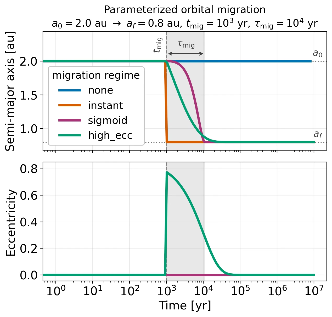
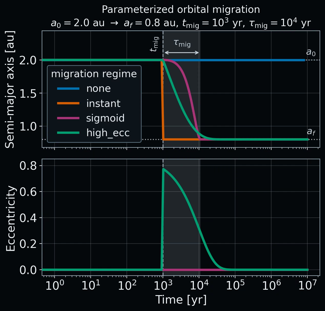
Semi-major axis (top) and eccentricity (bottom) for the four regimes, with
orbit.semimajoraxis = 2.0 au, sma_final = 0.8 au, time_migration = 1e3 yr and
tau_migration = 1e4 yr. The dashed vertical line marks the migration epoch
and the shaded band spans one tau_migration after it. The dotted horizontal
lines in the top panel mark the starting and final orbits, a_0 = orbit.semimajoraxis
and a_f = sma_final.
Planet-satellite models (orbit.planet_satellite_model)
| Model | Evolves | Reference | Notes |
|---|---|---|---|
ps0d |
semimajorax_sat, axial_period |
Korenaga (2023)5, Eq. 58-60 | No eccentricity evolution, no satellite-side tide. Uses the M_sat << M_planet limit of the orbital angular-momentum term (~1.2% error for Earth-Moon). |
ps1d |
axial_period, axial_period_sat, semimajorax_sat, eccentricity_sat, plan_sat_am |
Correia & Valente (2022)4 | Same vectorial approach as sp1d, extended to track both planet-raised and satellite-raised tidal contributions separately. Requires satellite-side Love-numbers (see below). |
ps1d_evec |
Everything ps1d evolves, plus evection_angle |
ps1d physics plus Rufu & Canup (2020)6 evection-resonance terms |
Adds a J2-driven apsidal-precession term and a resonant forcing term. See Evection resonance below. |
ps0d in a nutshell - Korenaga (2023)
Built to explain why the Moon's magma ocean stayed molten for so long: rather than solving the tidal potential in detail, it tracks one number, the system's total (spin + orbital) angular momentum, and lets the planet's tidal dissipation rate spend it. As the planet's spin winds down, the satellite's orbit must expand to keep the ledger balanced - a bookkeeping model, not a torque model, so it is cheap and exactly momentum-conserving, at the cost of no eccentricity evolution.
ps1d in a nutshell - Correia & Valente (2022)
The same Hansen-coefficient decomposition as sp1d, but with two
dissipating bodies instead of one: both the planet's and the
satellite's tidal responses pull on the shared orbit, so each of
their spins, the semi-major axis, and the eccentricity all evolve
together, coupled through one exchange of angular momentum.
ps1d_evec in a nutshell - Rufu & Canup (2020)
As a tidally-receding moon's orbit expands, its slow apsidal precession can fall into step with the star's apparent yearly motion - a secular resonance. Falling into that resonance is like pushing a swing at just the right moment: it pumps up the moon's eccentricity long after ordinary tides alone would have damped it flat, which is the paper's proposed route to the Moon's present-day orbital tilt.
Satellite Love-number lookup
Both ps1d and ps1d_evec need the satellite's own Love-number spectrum as a
function of forcing frequency, which only orbit.module='obliqua' can
supply (via LN_from_lookup).
Using ps1d/ps1d_evec unconditionally populates the satellite's tidal
parameters in tides_o through Obliqua's lookup_from_interior at the
start of the run.
Compatibility between orbit models and tidal modules
A tidal module makes up to two things available: the scalar
hf_row['Imk2'], and/or the full per-mode spectrum in tides_o. Which one
an orbit model reads is exactly what its 0d/1d suffix tracks -- a 0d
model reads the scalar path, a 1d model reads tides_o directly.
What each tidal module provides:
orbit.module |
Imk2 |
tides_o |
hf_row['F_tidal'] |
|---|---|---|---|
dummy |
Yes | No | Yes |
lovepy |
Yes | Yes | yes |
obliqua |
Yes, only when orbit.obliqua.n == [2] (0.0 otherwise) |
Yes, planet always, satellite too when orbit.perturber='satellite' |
yes |
What each orbit model reads:
| Model | Reads | Compatible orbit.module |
|---|---|---|
sp0d |
hf_row['Imk2'] |
dummy, lovepy, obliqua (requires orbit.obliqua.n == [2]) |
sp1d |
tides_o, (primary='planet', perturber='star') |
lovepy, obliqua |
parameterized |
-- | none (orbit.module = 'none' is required) |
ps0d |
hf_row['F_tidal'] |
dummy, lovepy, obliqua |
ps1d |
tides_o, (both primary='planet', perturber='satellite' and primary='satellite', perturber='planet') |
lovepy, obliqua |
ps1d_evec |
Same as ps1d, plus evection_angle |
lovepy, obliqua (Note that lovepy breaks down at high eccentricities, so it is not recommended for this case) |
Note on *1d models
sp1d, ps1d, and ps1d_evec are rejected at config load when
orbit.module is not 'obliqua' or 'lovepy'. Prefer
orbit.module='obliqua' for any *1d orbit model.
Satellite Love-number lookup (Obliqua only)
Unlike the planet, whose interior structure evolves and is re-queried
every coupling step, the satellite's interior is treated as static for
the lifetime of a run. orbit.obliqua.lookup_from_interior builds a full
frequency-spectrum Love-number table once, from a fixed satellite
interior description (orbit.satellite.love_number_sat, a JSON initial
condition read by a simplified 0-D solid/fluid Obliqua configuration),
and writes it to a NetCDF file (sat_tides.nc). Alternatively, the user
can provide their own pre-computed table (orbit.satellite.love_number_sat,
a NetCDF file), which will be used instead of the one generated by
lookup_from_interior. Every subsequent coupling step, LN_from_lookup
computes the satellite's own forcing frequencies from its current spin and
orbital state and interpolates the satellite's Love numbers from that fixed
table (linear in frequency, per tidal degree).
Evection resonance (ps1d_evec)
Evection resonance happens when a moon’s elongated orbit rotates at the
exact same speed that the central planet orbits its star.; capture into
it can pump the satellite's eccentricity well above
what tides alone would produce. ps1d_evec detects proximity to the
resonance location a'_res (Rufu & Canup 2020, Eq. 12) with a debounced,
hysteretic band detector (separate entry/exit margins,
orbit.solver.resonance_margin_enter/resonance_margin_exit, avoid
chattering at the band edge) and gates only the oscillating resonant
forcing term on that detector. The secular apsidal-precession term and
the evection angle's own evolution are always active regardless of
band status. Setting the gate to zero decouples the resonant forcing
term, reducing ps1d_evec to plain ps1d dynamics.
Example evection-resonance episode. The satellite starts outside the resonance band, evolving freely; capture into the band locks the evection angle to the resonant condition and pumps up the eccentricity; escape from the band later returns the system to free, non-resonant precession.
While in or near the band, two additional controls apply:
- Rate cap (
params.dt.evection_*): bounds the next PROTEUS coupling step so the fractional change ineccentricity_satstays nearevection_target_rel_de, since Obliqua's own adaptive spectrum window is chosen once per step from the eccentricity at that step's start. - Growth limiter: caps how fast the step size can grow relative to
the previous step while inside the band, or for
evection_cooldown_itersiterations after leaving it, so the coupling step does not snap back to its ordinary size the instant the band is exited.
Both are folded into the single exported column evection_dt_cap_yr,
which interior_energetics.timestep.next_step applies as one of several
caps on the next main-loop step.
Reproducing capture and peak eccentricity against Rufu & Canup (2020)
Figure 3 is validated in
tests/integration/test_slow_orbit_evection_ctl.py
(@pytest.mark.slow): the real ps1d_evec model, driven by a Mignard
constant-time-lag tidal spectrum, reproduces the paper's resonance-capture
timing window and peak-eccentricity location to better than 0.1% in
semi-major axis.
The "three clocks"
Fine-grained diagnostics for ps1d_evec (fine_evection_data.csv)
distinguish three different notions of "step":
- PROTEUS main-loop clock: one
evolve_orbit_satellitecall per coupling iteration, spanninginterior_o.dtyears. - Solver clock: the adaptive-substep controller's own internal
dt_yrsteps within one main-loop call (see below), and, within a single substep,solve_ivp's own internal integration points. - Storage clock: how densely those solver-clock samples are written
to disk. Every solver-clock sample is kept while inside the evection
band; outside the band, samples are thinned to a target spacing
(
orbit.solver.fine_csv_target_rel_dt, a fraction of the current main-loop step) so the file does not grow unbounded over a long, quiescent run.
Hansen coefficients
The sp1d/ps1d/ps1d_evec vectorial tidal models expand the tide-raising
potential in Hansen coefficients X_k^{n,m}(e), evaluated at every ODE
substep. A direct FFT evaluation is too slow for that (implicit solvers
probe many micro-varying eccentricities per step), and nearest-neighbor
caching would introduce discontinuities that break implicit solvers.
orbit.hansen instead pre-tabulates,
once per run, the eccentricity-dependent mode window [k_min, k_max]
(since the number of significant modes grows from ~10 near e=0 to
several hundred above e=0.8) and then the coefficient values themselves
on that window, both linearly interpolated in e thereafter. The tables
are warmed up once by orbit.wrapper.run_orbit at Time<=1; a hot-path
call lazily builds them if warm-up was skipped.
High eccentricity
The underlying Kepler solver does not converge beyond e~0.90, hence
a warning is issued.
Adaptive substep controller
sp1d, ps0d, ps1d, and ps1d_evec all integrate through the same
accept/reject controller,
orbit.common.run_adaptive_orbit_substeps.
For each attempted internal step it stages the tentative result, checks it
for unphysical values (negative semi-major axis, eccentricity outside [0, 1),
non-finite spin) and for excessive relative change in tracked quantities
(orbit.solver.max_rel_*), then either merges it in and grows the step,
or discards it and shrinks the step (orbit.solver.growth/shrink).
The same call also keeps the planet's moment of inertia (C_int, from
interior_energetics.common.get_C_planet)
consistent with the live interior structure: rather than jumping to the
freshly computed value once per call (which would put a discontinuity in
any quantity that depends on the planet's spin rate, such as ps1d_evec's
oblateness-driven precession), the controller ramps C_int linearly
across the call's accepted substeps, rescaling axial_period at each one
to conserve C_int * Omega_p (angular momentum).
ps0d additionally gets a cumulative drift cap: ps0d has no
eccentricity or spin feedback of its own, so many small, individually-legal
substeps can compound into a large silent migration within a single call.
Termination criteria
Orbital and rotational state feed three physical stopping conditions
(params.stop.*, checked in utils.terminate):
- Disintegration (
params.stop.disint/disint_sat): the planet or satellite orbiting within its partner's Roche limit, or spinning faster than its breakup rate. - Satellite escape (
params.stop.satellite): the satellite's semi-major axis exceedingsma_max.
Model selection guide
- Want a cheap, non-physical heat source for testing the interior's
response to tides?
orbit.module = 'dummy', no evolution model. - Want a self-consistent solid-body tidal response with minimal setup,
spin-orbit synchronised, low eccentricity?
orbit.module = 'lovepy'. - Want the planet's orbit and spin to evolve self-consistently with its
own interior structure, at arbitrary eccentricity?
orbit.module = 'obliqua',orbit.perturber = 'star',orbit.star_planet_model = 'sp1d'. - Want a fast, closed-form estimate of star-planet tidal circularisation
without resolving spin?
orbit.module.dummysupplyingImk2plusorbit.star_planet_model = 'sp0d'. - Want a satellite's orbit (e.g. a moon) to evolve, including its own
tidal response?
orbit.module = 'obliqua',orbit.perturber = 'satellite',orbit.planet_satellite_model = 'ps1d'(or'ps0d'for a cheaper, eccentricity-frozen estimate). - Want to also study capture into, and eccentricity pumping by, the
evection resonance?
orbit.module = 'obliqua',orbit.perturber = 'satellite',orbit.planet_satellite_model = 'ps1d_evec'.
Testing
- Unit tests (
tests/orbit/*.py,@pytest.mark.unit) mock Julia calls forlovepy/obliquaand pin closed-form results forsp0d,sp1d,ps0d,ps1dagainst their source papers, each with a discrimination guard against the nearest plausible wrong formula (wrong exponent, wrong sign, or the wrong mass in a prefactor). Angular momentum conservation forsp1d/ps1dis checked directly, both as a raw total and as a targeted spin-vs-orbital exchange test sized to catch a bug the raw total alone would miss. - Slow/integration tests (
tests/integration/test_slow_orbit_evection_ctl.py,@pytest.mark.slow) drive the realps1d_evecmodel end-to-end and compare against the published Rufu & Canup (2020) evection trajectory. - Per-source-file test inventories, references, and re-derivations are
tracked under
docs/Validation/orbit/:orbit.py,satellite.py,wrapper.py,obliqua.py.
See also: Model description | Star and orbit configuration | Execution and output configuration | Validation: orbit
-
van Dijk, M.R., Nicholls, H. & Lichtenberg, T., Onset of Habitable Conditions on the Hadean Earth Set by Feedback between Tides and Greenhouse Forcing, The Planetary Science Journal, 7, 94, 2026. ↩
-
Nicholls, H., Guimond, C.M., Hay, H.C.F.C., Chatterjee, R.D., Lichtenberg, T. & Pierrehumbert, R.T., Self-limited tidal heating and prolonged magma oceans in the L 98-59 system, Monthly Notices of the Royal Astronomical Society, 541, 2566-2584, 2025. ↩
-
Driscoll, P. & Barnes, R., Tidal Heating of Earth-like Exoplanets around M Stars: Thermal, Magnetic, and Orbital Evolutions, Astrobiology, 15, 739, 2015. ↩
-
Correia, A.C.M. & Valente, E.F.S., A simple model to study tides in moons, Celestial Mechanics and Dynamical Astronomy, 134, 27, 2022. ↩↩
-
Korenaga, J., Rapid tidal dissipation explains the extended lunar magma ocean, Icarus, 400, 115564, 2023. ↩
-
Rufu, R. & Canup, R.M., Evection resonance as a possible cause for lunar inclination, Journal of Geophysical Research: Planets, 125, e2019JE006312, 2020. ↩
-
Postolec, E., Lichtenberg, T., Teske, J.K., Nicholls, H., Attia, M., Piette, A., Dang, L., Wallack, N.L., Plotnykov, M., McGinty, A., Boucher, S., Peng, B. & Valencia, D., Evolutionary pathways toward survival of a thick CO2- or SO2-rich atmosphere on the lava world TOI-561 b, submitted to The Astrophysical Journal, arXiv:2609.03144, 2026. ↩↩