Mass-radius relation
What this page checks
This page checks the full structure solver of Zalmoxis: the radius, the central pressure and the gravity of a planet of given mass and core mass fraction (CMF, the mass fraction of the iron core). The cases run the full solver with the Seager et al. (2007) analytic equation of state (EOS) and compare the planet with the Earth, published scaling laws and physical trends. Validation means that a test runs the code on a case with a known right answer and checks the result within a stated tolerance. If the solver is wrong, every planet radius and interior profile of Zalmoxis is wrong. Each case below says why the check exists, what it tests, how we know the right answer and why it matters, and ends with a box "Test details". The overview lists every case of the tab.
Earth benchmark
Why this check exists. The solver has 3 nested loops: the mass-radius convergence, the Picard iteration of the density and the Brent root search of the central pressure. A gross error in any loop can still give a converged but wrong planet, without an error message; the case catches it only when it takes the radius, the surface gravity or the central pressure outside its wide tolerance (5, 10 and 15 %).
What it tests. The complete solver chain against the best-known planet in the solar system. Setup: planet mass \(M_p = 1\, M_\oplus\), core mass fraction \(f_c = 0.325\), Seager et al. (2007) analytic EOS (iron core, MgSiO\(_3\) mantle). No tabulated data files needed. The analytic EOS uses the modified polytrope \(\rho(P) = \rho_0 + c P^n\) with published coefficients.
The results:
| Quantity | Zalmoxis | Earth | Deviation |
|---|---|---|---|
| Radius | 6114.5 km | 6371 km | 4% below |
| Central pressure | 391 GPa | 365 GPa | 7% above |
| Surface gravity | 10.67 m/s\(^2\) | 9.81 m/s\(^2\) | 9% above |
The test compares the radius with the Earth radius of zalmoxis.constants, 6335.4 km: 6114.5 km is 0.965 of that value.
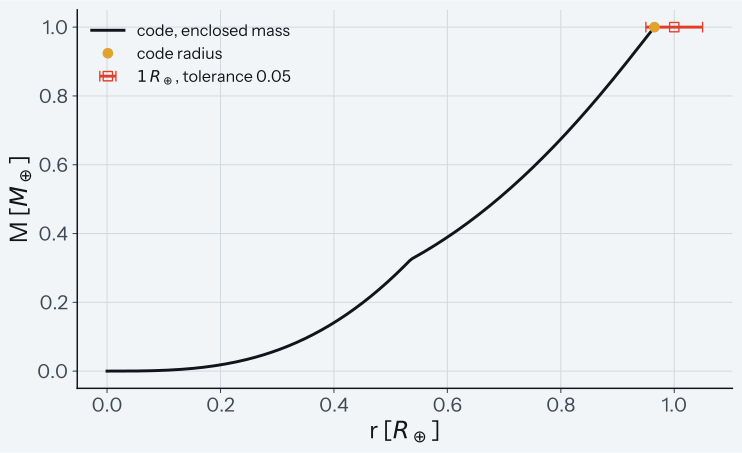
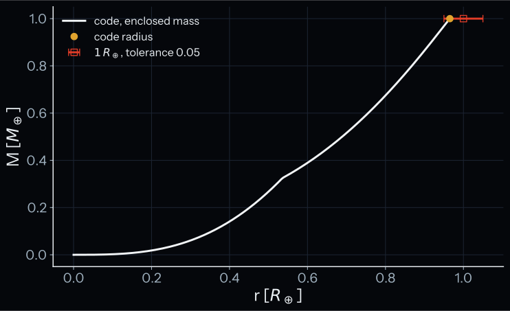
How to read the plot. The line is the enclosed mass of the 1 Earth-mass solve against radius and gives context. The radius test asserts the planet radius (circle) against \(1\,R_\oplus\) (square, with the horizontal error bar 0.05). A pass means that the circle lies inside the error bar.
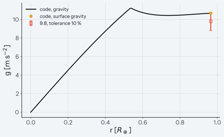
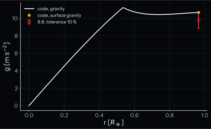
How to read the plot. The line is the gravity of the same solve. The gravity test asserts the surface gravity (circle) against 9.8 m/s\(^2\) (square, with its error bar of 10 %). The circle, 10.67 m/s\(^2\), lies close to the upper end of the bar, 10.78 m/s\(^2\). A pass means that the circle lies inside the error bar.
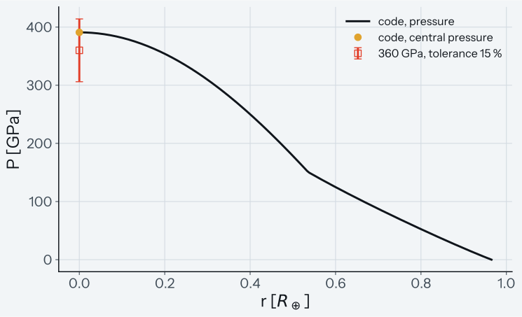
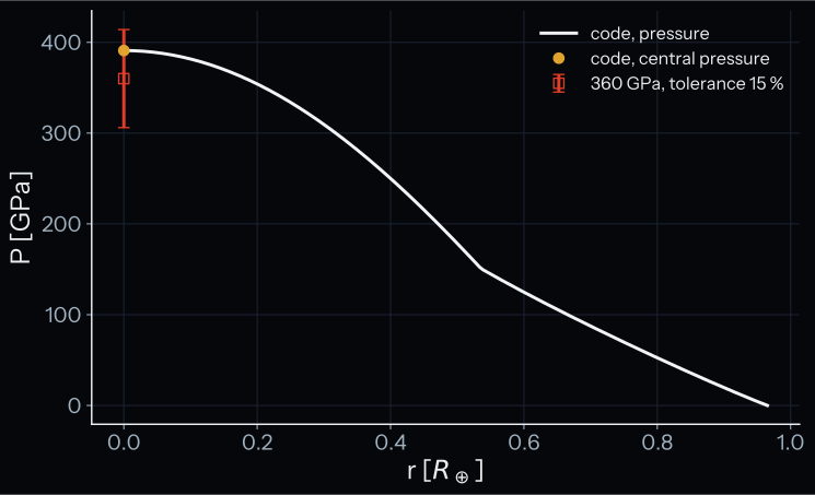
How to read the plot. The line is the pressure of the same solve. The pressure test asserts the central pressure (circle) against 360 GPa (square, with its error bar of 15 %). A pass means that the circle lies inside the error bar.
How we know the right answer. The radius and surface gravity of the Earth, and its central pressure from models (360 GPa in the test; zalmoxis.constants cites 365 GPa from Nimmo 2015). The 4-9% deviations are expected and physically understood. The Seager modified polytrope is a temperature-independent, zero-Kelvin EOS fit to the merged Vinet/Birch-Murnaghan (low pressure) and Thomas-Fermi-Dirac (high pressure) equations of state. It does not account for thermal expansion, which makes real Earth's mantle less dense (and therefore larger) than the zero-temperature prediction. In this solve the density jumps at the core-mantle boundary at about 3380 km radius, with iron densities of 11,100-12,900 kg/m\(^3\) in the core and silicate densities of 4,100-5,900 kg/m\(^3\) in the mantle. The gravity peaks at the CMB, at about 11.2 m/s\(^2\), falls to about 10.4 m/s\(^2\) near 4700 km and rises again to 10.67 m/s\(^2\) at the surface. No assert checks these profile values; only the surface gravity is asserted.
Why it matters. This case checks all 3 loops of the solver at once.
Known limit. The tolerances are wide (radius 5 %, gravity 10 %, central pressure 15 %), because the zero-temperature EOS is 4-9 % from the Earth. A loop error that moves the radius by about 1 % passes this case.
Test details
- Reference: Earth values as the test pins them: radius \(1\,R_\oplus\), surface gravity 9.8 m/s\(^2\), central pressure 360 GPa (the test names no source; the table above compares with 6371 km, 9.81 m/s\(^2\) and 365 GPa)
- Tolerance: radius to
abs=0.05of \(1\,R_\oplus\), surface gravity torel=0.10of 9.8 m/s\(^2\), central pressure torel=0.15of 360 GPa - Test id:
tests/test_first_principles.py::TestEarthBenchmark - Command:
pytest -o "addopts=" tests/test_first_principles.py::TestEarthBenchmark
Mass-radius scaling and CMF sensitivity
Why this check exists. A solver can match one planet and still give wrong trends with mass or composition. Gross errors in a trend fail these checks; the exponent test accepts 0.23 to 0.31, so a small slope error passes.
What it tests. Whether the solver gives physically correct trends across parameter space, not just a single point: the mass-radius relation, the radius against the CMF, and conservation checks.
Mass-radius relation
For rocky planets with Earth-like composition, the mass-radius relation follows an approximate power law \(R \propto M^\alpha\) where \(\alpha \approx 0.27\) (Seager et al. 2007). The exponent is less than \(1/3\) (the value for an incompressible sphere of constant density) because larger planets have higher internal pressures that compress the material, partially offsetting the volume increase from added mass.
Running Zalmoxis from 0.3 to 10 \(M_\oplus\) with \(f_c = 0.325\) and fitting \(\log R\) vs \(\log M\) gives \(\alpha = 0.293\) (the test fits 0.5 to 10 \(M_\oplus\) and gets 0.289). The plot shows the solves of the test.
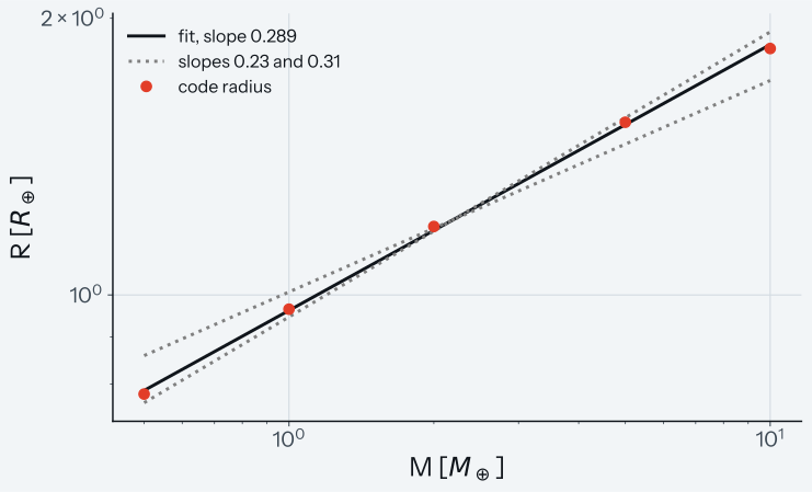
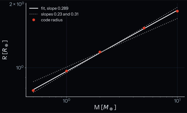
How to read the plot. Both axes are logarithmic. The circles are the code radii of the 5 solves at 0.5, 1, 2, 5 and 10 Earth masses. The solid line is their least-squares fit, with exponent \(\alpha\) = 0.289. The dotted lines have the exponents 0.23 and 0.31, the edges of the asserted range \(0.27 \pm 0.04\), drawn through the centre of the fit. A pass means that the exponent of the solid line lies between those of the dotted lines.
The fitted exponent is slightly higher than the Seager et al. value of 0.27, which reflects the sensitivity of the power-law fit to the mass range used. Seager et al. fit over 1-10 \(M_\oplus\), where Zalmoxis gives 0.284; including sub-Earth masses (0.3 \(M_\oplus\)) steepens the slope because low-mass planets are less compressed, making the \(R(M)\) curve slightly steeper at the low-mass end.
CMF monotonicity
At fixed mass (\(1\, M_\oplus\)), increasing the core mass fraction (replacing less dense silicate with denser iron) must monotonically decrease the radius. This is a basic physical constraint: iron (\(\rho_0 = 8300\) kg/m\(^3\)) is roughly twice as dense as MgSiO\(_3\) (\(\rho_0 = 4100\) kg/m\(^3\)), so more iron means a more compact planet.
Zalmoxis produces a strictly decreasing curve from \(R \approx 1.02\, R_\oplus\) at \(f_c = 0.05\) (nearly pure silicate) to \(R \approx 0.81\, R_\oplus\) at \(f_c = 0.95\) (nearly pure iron), in units of the 6335.4 km Earth radius of zalmoxis.constants. The plot shows the solves of the test.
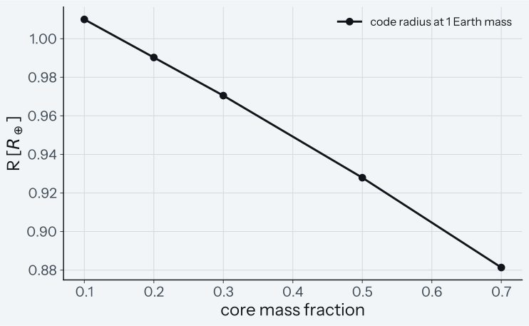
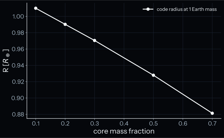
How to read the plot. The circles joined by the line are the code radii of 1 Earth-mass planets at the core mass fractions 0.1, 0.2, 0.3, 0.5 and 0.7. The test asserts that each radius is smaller than the one before. A pass means that the line falls at every step.
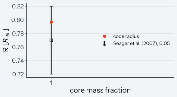
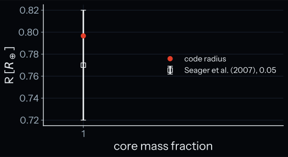
How to read the plot. The pure-iron test asserts the code radius of a pure iron planet (circle) against \(0.77\,R_\oplus\) (square). The square is the Seager et al. (2007) value, with its error bar of 0.05. A pass means that the circle lies inside the error bar; it lies at \(0.80\,R_\oplus\).
A pure iron planet (\(f_c = 1\)) has \(0.80\, R_\oplus\), against the Seager et al. (2007) value of \(0.77\, R_\oplus\) for a 1 \(M_\oplus\) iron planet; the test accepts abs=0.05. The radius falls faster with CMF at high CMF: by 0.043 \(R_\oplus\) from \(f_c = 0.3\) to 0.5 and by 0.047 \(R_\oplus\) from 0.5 to 0.7.
Conservation checks on full solver output
The smoke tests of TestConservationLaws also verify three conservation properties of the full solver output:
- Mass conservation: \(M(R_\mathrm{surface}) = M_p\) to 1 %, and to 2 % by trapezoidal integration of \(4\pi r^2 \rho(r)\) over the solver's own density and radii.
- Surface pressure: \(P(R_\mathrm{surface}) = P_\mathrm{target}\) (101,325 Pa) to 2 GPa, twice the default surface-pressure tolerance of the solver (1 GPa).
- Gauss's law: the integrated \(g\) equals \(GM/r^2\) to \(< 10^{-3}\) relative error at every radius except the first 6 grid points and the points with \(P \leq 0\).
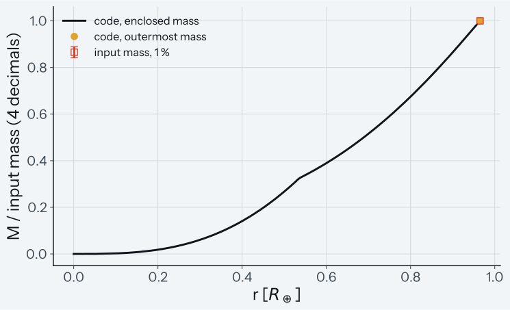
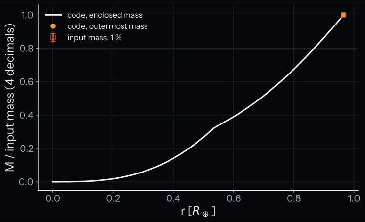
How to read the plot. The line is the enclosed mass of the solve over the input mass, to 4 decimals, against radius. The mass test asserts the outermost mass (circle) against the input mass (square, with its error bar of 1 %). A pass means that the circle lies inside the error bar.
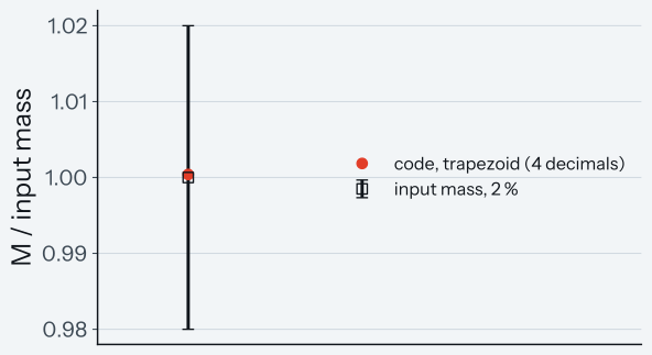
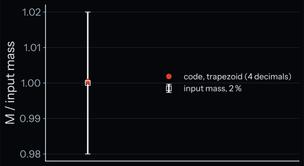
How to read the plot. The trapezoid test integrates \(4\pi r^2 \rho\) over the radius with the trapezoidal rule. It asserts the result (circle, to 4 decimals) against the input mass (square, with its error bar of 2 %). A pass means that the circle lies inside the error bar.
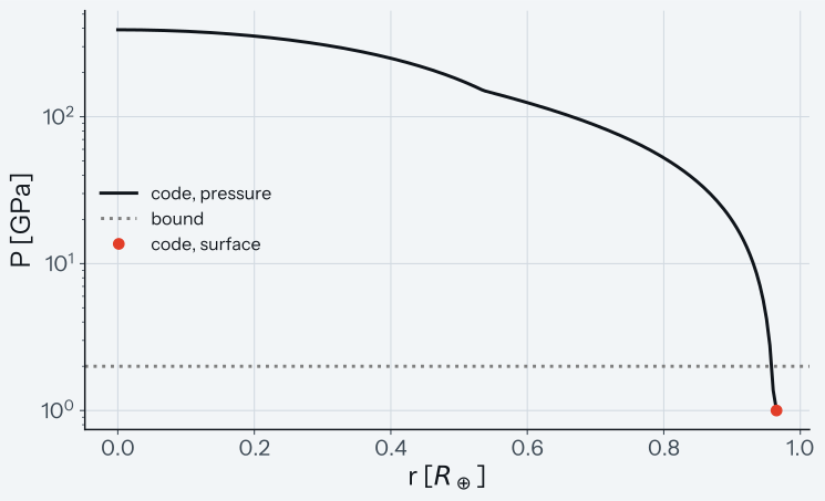
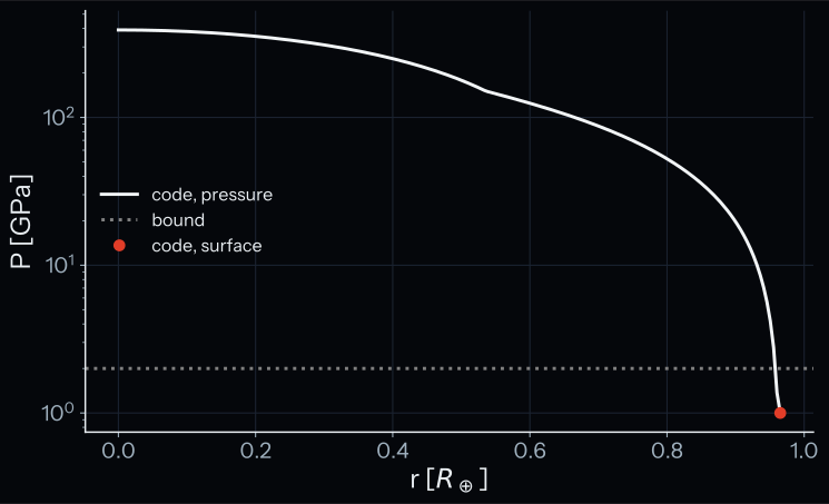
How to read the plot. The line is the pressure of the solve on a log axis. Pressures below 1 GPa are drawn at 1 GPa, so that the plot is the same on every platform. The surface value itself is about \(10^5\) Pa. The surface-pressure test asserts that it differs from 101325 Pa by less than 2 GPa (dotted line). A pass means that the surface circle lies below the dotted line.
Known limit. The surface-pressure check allows 2 GPa against a target of 101,325 Pa, so it cannot tell a correct surface pressure from one 10000 times too large. The solver treats a residual below 1 GPa as pressure-converged, but it can also accept a solution on mass convergence alone, so this 2 GPa check is then the only guard. The mass checks allow 1 % and 2 %.
How we know the right answer. The scaling law and the pure-iron radius of Seager et al. (2007), and physical constraints (monotonicity, mass, surface pressure, Gauss's law) with no published reference.
Why it matters. These trends are what a grid of Zalmoxis planets depends on.
Test details
- Reference:
TestMassRadiusScaling, \(\alpha \approx 0.27\) for masses 0.5, 1, 2, 5 and 10 \(M_\oplus\), andTestPureIronPlanet, \(0.77\,R_\oplus\) for CMF = 1.0, both from Seager et al. (2007);TestCMFMonotonicity(CMF 0.1 to 0.7) andTestConservationLawscheck physical constraints with no published reference - Tolerance: exponent to
abs=0.04of 0.27; strictly decreasing radius with CMF; pure-iron radius toabs=0.05of \(0.77\,R_\oplus\); mass within 1% (2% by trapezoidal integration); surface pressure at most 2e9 Pa from the target; Gauss's lawrtol=1e-3 - Test id:
tests/test_first_principles.py::TestMassRadiusScaling,tests/test_first_principles.py::TestCMFMonotonicity,tests/test_first_principles.py::TestPureIronPlanet,tests/test_first_principles.py::TestConservationLaws - Command:
pytest -o "addopts=" tests/test_first_principles.py::TestMassRadiusScaling tests/test_first_principles.py::TestCMFMonotonicity tests/test_first_principles.py::TestPureIronPlanet tests/test_first_principles.py::TestConservationLaws
Reproducing the results
The tests draw the plots of these cases. This command writes them again to docs/assets/validation/:
pytest -o "addopts=" tests/test_first_principles.py tests/test_polytrope_verification.py --validation-plots
Without --validation-plots the tests write nothing: each compares the data of its plot with the committed pair, and a missing or stale file fails the test.