Hydrostatic structure

What this page checks

This page checks how Zalmoxis computes the inside of a planet in hydrostatic equilibrium: the mass, the gravity and the pressure at each radius. Validation here means that we run the code on a case where another source gives the right answer. The test then checks that the code gives that answer within a stated tolerance. The right answer comes from closed-form solutions, from conservation laws, from a second implementation of the same equations, or from the pressure that the planet must have at its surface. If this part of the code is wrong, every structure that Zalmoxis returns is wrong. This holds also for the structures it gives to PROTEUS: the radius of the planet and the pressure and gravity at each depth. Each case below says why the check exists, what it tests, how we know the right answer and why it matters. The box "Test details" at the end of each case gives the reference, the tolerance, the test id and the command. The overview lists every case of the tab.

Terms of this page.

• \(r\) and \(R\): the radius, from 0 at the centre, and the outer radius of the planet.
• \(R_\oplus\): the Earth radius of zalmoxis.constants, 6335.4 km (the mean Earth radius is 6371 km); \(M_\oplus\): the Earth mass, \(5.972 \times 10^{24}\) kg.
• \(M(r)\), \(g(r)\), \(P(r)\), \(\rho(r)\): the mass inside radius \(r\) (the enclosed mass, kg), the gravitational acceleration (m/s\(^2\)), the pressure (Pa) and the density (kg/m\(^3\)) at radius \(r\); \(G\) is the gravitational constant.
• EOS (equation of state): the relation \(\rho(P, T)\) between the density, the pressure and the temperature of a material.
• CMB: the core-mantle boundary. \(\rho_c\): the density at the centre.
• ODE integrator: the code that steps the three structure equations (ordinary differential equations) outward in \(r\).
• \(N\) and rtol: the number of radial grid points, and the relative tolerance of the ODE integrator (RK45, an adaptive Runge-Kutta method of order 4 and 5); the configuration key is relative_tolerance.
• Relative error: \(|x_\mathrm{num} - x_\mathrm{exact}| / |x_\mathrm{exact}|\), the difference between the computed and the exact value, divided by the exact value.
• Round-off level: a relative error of about \(10^{-16}\) to \(10^{-13}\), the size of the rounding error of floating-point arithmetic. A result at this level is exact within the precision of the computer.
• Central pressure \(P_c\): the pressure at the centre of the planet.
• Pressure solve: the loop that adjusts \(P_c\) until the pressure at the outer radius equals the target surface pressure \(P_t\) (written \(P_\mathrm{target}\) on the process-flow page).
• Brent's method (scipy.optimize.brentq): the root finder of the pressure solve. It narrows a bracket around a sign change of the residual and stops when the bracket is narrower than xtol, \(10^6\) Pa in the pressure solve. Newton's method, used by the Newton outer solver, instead steps towards the zero of a function along its slope.
• Residual \(f(P_c) = P(R) - P_t\): the pressure \(P(R)\) at the outer radius \(R\) minus the target surface pressure \(P_t\).
• Target surface pressure \(P_t\): 1 atm, 101325 Pa, unless a case says otherwise.
• Reached: the integration from a trial \(P_c\) reaches the outer radius.
• Surface stop: the integration ends where the pressure reaches 0 before the outer radius.
• Miss: \(\lvert P(R) - P_t \rvert\), often given in units of \(P_t\).
• Converged: the outer solver met one of its accept tests; accepted_on names the test.
• Relative planet-mass change: a change of the planet mass divided by the planet mass, for example \(10^{-9}\).
• Padded: the integration stops before the outer radius, and the remaining nodes, the padded nodes, get zero pressure. The residual is then \(-P_t\).
• Sign pair: 2 neighbouring evaluated central pressures, with a finite negative residual at the lower one and a finite positive residual at the higher one, so \(f\) changes sign between them. The higher one is the reached end.
• PALEOS: the tabulated equations of state for iron, MgSiO\(_3\) and water that Zalmoxis uses as its standard (EOS physics).
• Unified and 2-phase PALEOS mantle: one table for all phases of MgSiO\(_3\) (unified), or separate tables for the solid and the melt (2-phase). The mushy zone factor sets the solidus as a fraction of the liquidus (0.8 in the JAX cases).
• Wet mantle: a mantle with a dissolved volatile, here 1 % PALEOS H\(_2\)O.
• State (JAX cases): one set of \(r\), \(M\), \(g\) and \(P\) at which both codes evaluate the right-hand side.
• JAX path: an optional version of the structure integration in JAX, a Python library for compiled numerical code; it is off by default.
• Picard outer solver: the default outer loop. It solves the structure for a trial radius, compares the computed mass with the planet mass, and rescales the radius.
• Newton outer solver: the outer loop with Newton steps and a Brent fallback (outer_solver = 'newton'); PROTEUS uses it by default. It needs relative_tolerance at or below \(10^{-7}\).
• Newton tolerance (newton_tol, default \(10^{-4}\)): the Newton outer solver accepts a structure when its relative mass error is below this value and its pressure solve converged (accepted_on = 'newton_tol').

Governing equations

Every case on this page checks one part of the solution of these equations. Zalmoxis solves three coupled ordinary differential equations (ODEs) for the radial structure of a self-gravitating, spherically symmetric body in hydrostatic equilibrium:

The first equation adds the mass of each thin shell, the second is the derivative of \(g = GM/r^2\), and the third says that the pressure falls outward by the weight of the material above. The integration runs outward from the centre (\(r = 0\)) with the initial conditions \(M(0) = 0\), \(g(0) = 0\) and \(P(0) = P_c\).

The gravity equation is singular at \(r = 0\) because of the \(2g/r\) term. L'Hopital's rule gives the limit \(dg/dr|_{r=0} = \frac{4}{3}\pi G \rho_c\), and coupled_odes in zalmoxis.structure_model uses this limit at \(r = 0\).

An equation of state \(\rho = \rho(P, T)\) closes the system. The uniform-sphere, two-layer, conservation and binding-energy cases, and the uniform-sphere part of the grid and tolerance checks, fix \(\rho\) to a constant. The n = 1 polytrope case uses \(P = K\rho^2\). The full-solver part of the grid and tolerance checks, and the Earth benchmark and the mass-radius scaling on the mass-radius page, use the Analytic EOS, the modified polytrope of Seager et al. (2007), \(\rho(P) = \rho_0 + c P^n\), with fitted constants \(\rho_0\), \(c\) and \(n\) for each material (this \(n\) is not the index of the \(n = 1\) polytrope). None of these needs table data; the JAX table cases, the PALEOS Newton setups and the PALEOS setups of the sweep figure use the PALEOS tables.

Uniform-density sphere

Why this check exists. The integrator of the three equations must use the right coefficients and signs. A wrong factor in \(dM/dr\) or \(dg/dr\) (for example \(2\pi\) in place of \(4\pi\), or \(g/r\) in place of \(2g/r\)), or the wrong sign of \(dP/dr\), makes the computed mass, gravity or pressure differ from the exact solution, and this test fails.

What it tests. The density is fixed: the test replaces calculate_mixed_density() by a function that returns a constant \(\rho\), so no EOS table is used and only the RK45 integration of the three equations is tested. The setup is \(\rho = 5000\) kg/m\(^3\) (an average rocky planet), \(R = 6.4 \times 10^6\) m (about \(1\, R_\oplus\)), \(P_c = 360\) GPa, \(N = 300\) radial grid points and rtol \(= 10^{-10}\). The test makes six checks:

1. Mass profile: \(|M_\mathrm{num} - M_\mathrm{exact}| / M_\mathrm{exact} < 10^{-6}\) at all \(r > 0\).
2. Gravity profile: \(|g_\mathrm{num} - g_\mathrm{exact}| / g_\mathrm{exact} < 10^{-6}\) at all \(r > 0\).
3. Pressure profile: \(|P_\mathrm{num} - P_\mathrm{exact}| / P_\mathrm{exact} < 10^{-6}\) where \(P > 0\).
4. Central boundary conditions: \(M(0) = 0\), \(g(0) = 0\) and \(P(0) = P_c\) to machine precision.
5. Gravity slope at the centre: the slope of the computed gravity over the first two grid steps matches \(\frac{4}{3}\pi G \rho\) to \(< 10^{-4}\). This is the slope that the integration produces, not the value that coupled_odes uses at \(r = 0\).
6. Pressure monotonicity: \(dP/dr < 0\) everywhere \(P > 0\), as hydrostatic equilibrium requires with positive density and gravity.

How we know the right answer. For a sphere of constant density the equations have an exact closed-form solution, a textbook result with no free parameters:

The mass grows as \(r^3\) (the volume of a sphere), gravity is linear in \(r\) (Gauss's law for a uniform sphere), and the pressure falls as a parabola (hydrostatic equilibrium with a gravity that grows linearly).

Why it matters. Every structure that Zalmoxis returns comes from this integrator. An error here enters every profile, for every equation of state.

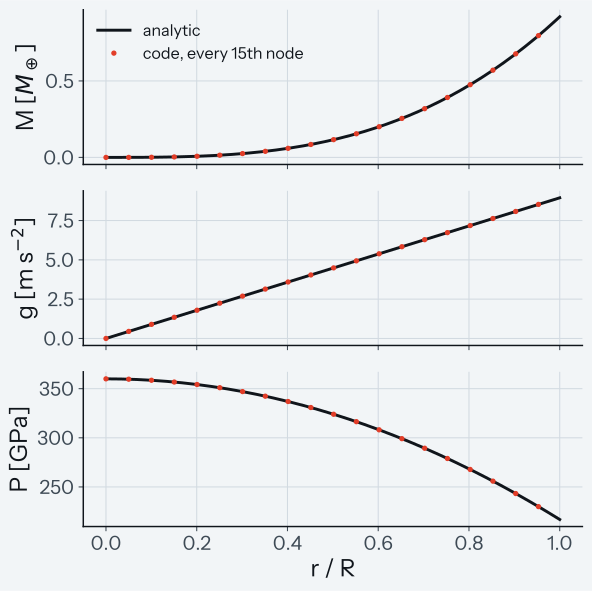
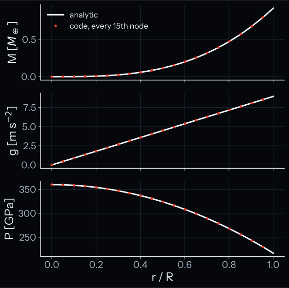
How to read the plot. The 3 panels show the enclosed mass, the gravity and the pressure against \(r/R\). The lines are the analytic solution and the marks are the code values, every 15th node. The tests of the class assert all 3 profiles against the analytic solution to a relative tolerance of \(10^{-6}\), too small to see. The pressure test draws the plot and asserts its pressure panel. The mass and gravity panels come from a second solve in the plot code; the mass and gravity tests assert them. A pass means that every mark lies on its line. The tests of the centre values and of the falling pressure are not drawn.

Known limit. This test does not check the value of the centre limit of \(dg/dr\): when coupled_odes uses \(\pi G \rho_c\) in place of \(\frac{4}{3}\pi G \rho_c\) at \(r = 0\), every test of the uniform-sphere, two-layer, conservation and binding-energy cases, the grid and tolerance checks and the \(n = 1\) polytrope case still passes.

Two-layer sphere

Why this check exists. Zalmoxis assigns each radial shell to a layer (core or mantle) by the enclosed mass. If this assignment is wrong, for example if the core ends at 90 % of its mass, the mass profile differs from the piecewise exact solution and this test fails. Wrong coefficients in \(dM/dr\) or \(dg/dr\) also make it fail.

What it tests. A sphere of two layers with constant densities: \(\rho_\mathrm{core} = 13{,}000\) kg/m\(^3\) (an iron-like core) and \(\rho_\mathrm{mantle} = 4000\) kg/m\(^3\) (a silicate-like mantle), with planet mass \(M_p = 1\, M_\oplus\) and core mass fraction \(f_c = 0.325\). The density jumps at the core-mantle boundary (CMB), the sharpest feature that the integrator must handle. The CMB radius is

This is close to the Earth's CMB radius of 3480 km, and the planet radius is 6513 km (1.03 \(R_\oplus\), or 1.02 times the mean Earth radius of 6371 km). The central pressure of this profile, 380 GPa, comes from integrating the hydrostatic equation over the known density profile. The integration starts 5 % above it, at 399 GPa, so that the pressure stays positive out to the surface. The test compares the enclosed mass with the exact solution and checks Gauss's law (\(g = GM/r^2\)) in both layers.

How we know the right answer. With two constant densities, the enclosed mass has an exact piecewise solution:

Why it matters. Every Zalmoxis planet has at least a core and a mantle. A wrong layer boundary puts the wrong material at a radius, so the density, the radius and the pressure at the CMB are wrong.

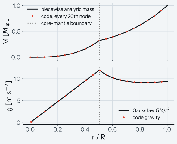
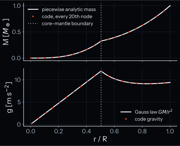
How to read the plot. The top panel shows the piecewise analytic mass (line) and the code mass (marks, every 20th node). The bottom panel shows \(GM/r^2\) from the code mass (line) and the code gravity (marks). The dotted line is the core-mantle boundary. This test asserts the mass to a relative tolerance of \(10^{-5}\), too small to see. The bottom panel comes from a second solve in the plot code. The Gauss's law test asserts it to \(10^{-4}\) on the same setup. A pass means that every mark lies on its line.

Conservation diagnostics

Why this check exists. Zalmoxis integrates \(M(r)\) and \(g(r)\) as two separate ODE components; it does not compute \(g\) from \(M\). A wrong factor in \(dM/dr\) or \(dg/dr\) makes them disagree, and the Gauss's law check fails. A wrong sign of \(dP/dr\) breaks hydrostatic balance, and the balance check fails.

What it tests. Two conservation laws must hold at every point of any physically consistent solution, for any EOS. The test checks them on the uniform-density sphere above.

• Gauss's law: \(g(r) = G\,M(r) / r^2\) for all \(r > 0\). The relative residual \(|g - GM/r^2| / (GM/r^2)\) measures how far the two integrated components drift apart.
• Hydrostatic balance: \(dP/dr + \rho\, g = 0\) at every interior point. This is the defining equation of the solver. The test computes \(dP/dr\) by central finite differences and divides the residual by \(P_\mathrm{scale} = \frac{2}{3}\pi G \rho^2 R\), a pressure gradient scale in Pa/m. For the uniform sphere \(P(r)\) is a parabola, so the central difference is exact and the residual shows the integration error alone.

How we know the right answer. Gauss's law and hydrostatic balance follow from the equations themselves, so the exact residual is zero.

Why it matters. These laws must hold for every planet that Zalmoxis computes, also where no closed-form solution exists.

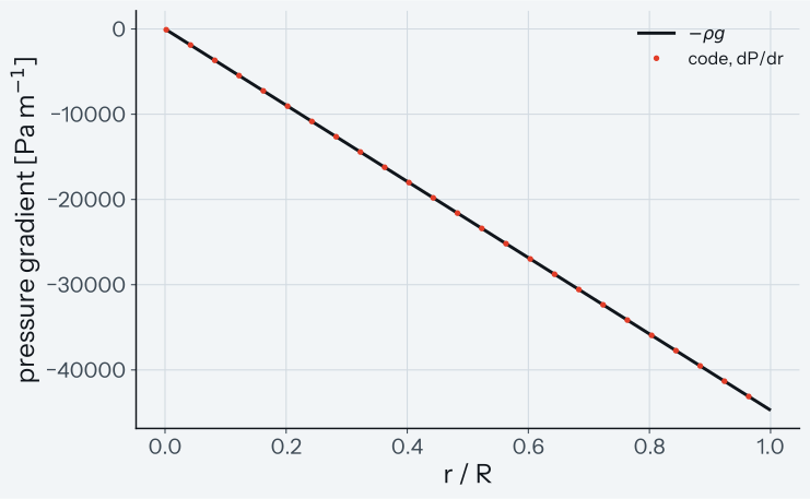
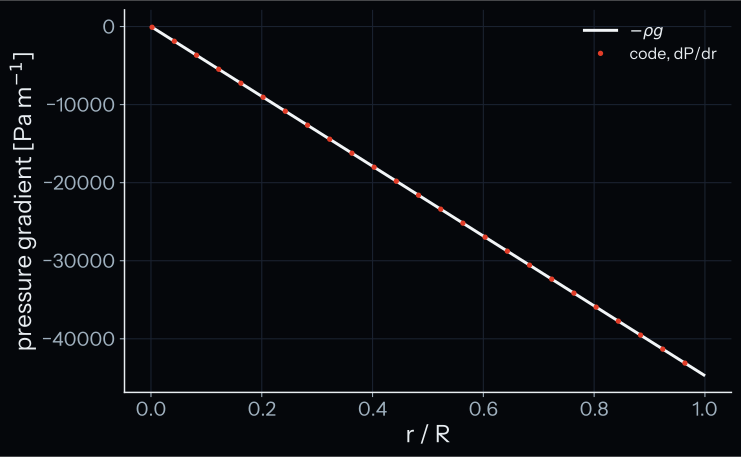
How to read the plot. The line is \(-\rho g\) and the marks are the code \(dP/dr\) by central differences, every 20th interior node, against \(r/R\). The balance test asserts that their difference stays below \(10^{-4}\) of the gradient scale \(\frac{2}{3}\pi G \rho^2 R\). The difference is round-off, at most \(1.5 \times 10^{-13}\) of that scale, so the marks lie on the line. A pass means that every mark lies on the line.

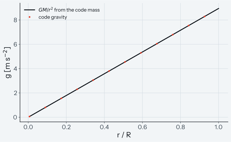
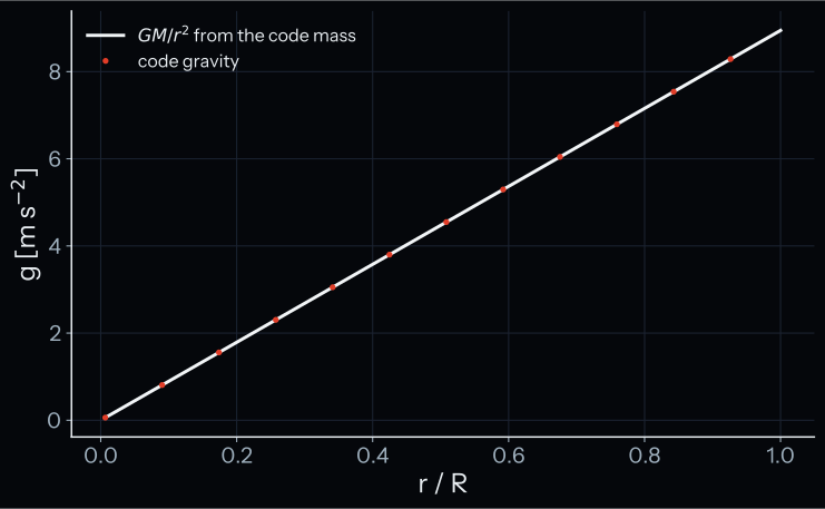
How to read the plot. The line is \(GM/r^2\) from the code mass and the marks are the code gravity, every 25th node, on the 300-point grid. The Gauss's law test asserts that they agree to a relative tolerance of \(10^{-5}\), too small to see. A pass means that every mark lies on the line.

Gravitational binding energy

Why this check exists. The cases above check the profiles point by point. An integral over the whole planet checks that the mass and density profiles agree as a whole. A wrong factor in \(dM/dr\) makes this test fail.

What it tests. The gravitational binding energy \(E_\mathrm{grav}\) [J], the energy needed to disperse the planet to infinity, is

The test integrates it with the trapezoidal rule over the \(M(r)\) and \(\rho(r)\) profiles of the uniform-density sphere (\(N = 500\)).

How we know the right answer. For uniform density the integral has the closed form \(E_\mathrm{grav} = -\frac{3}{5}\, G\, M_p^2 / R\). The numerical value agrees with it to \(7 \times 10^{-6}\); the test asserts \(< 1\%\).

Why it matters. The binding energy integrates the whole profile, so an error that adds up over the planet shows here even when each point looks right.

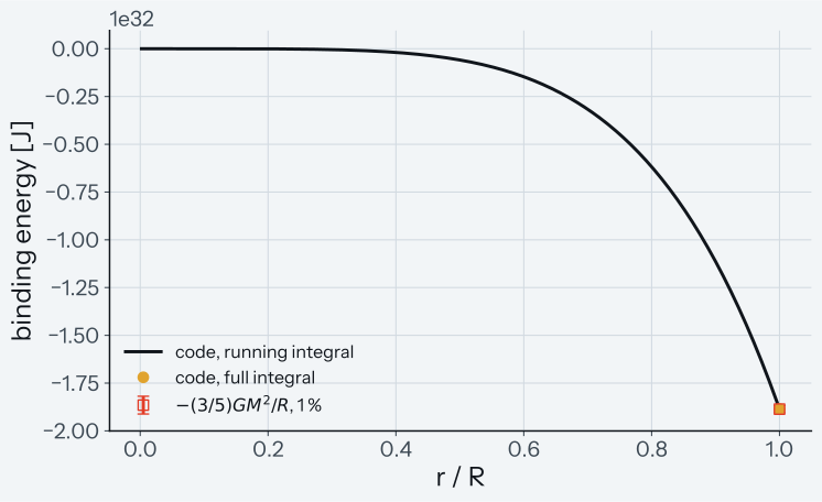
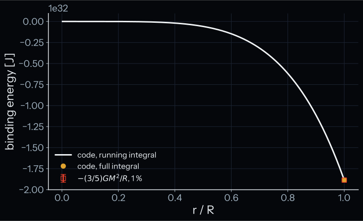
How to read the plot. The line shows how the binding-energy integral builds up from the centre outward, from the code mass profile; it is not asserted. The test asserts the full integral (circle) against \(-\frac{3}{5} G M_p^2 / R\) (square, with its error bar of 1 %). A pass means that the circle lies inside the error bar.

The Earth benchmark and the mass-radius scaling are on the mass-radius page.

n = 1 polytrope

Why this check exists. The first 4 cases on this page fix the density. This case lets the density follow the pressure through an equation of state, as in a real planet. A wrong factor in \(dM/dr\) or \(dg/dr\), or the wrong sign of \(dP/dr\), moves the surface radius or the integrated mass, and the test fails.

What it tests. solve_structure with the Analytic:polytrope_n1 verification material, \(P = K \rho^2\) (a polytrope of index \(n = 1\), with \(K\) a constant in Pa m\(^6\) kg\(^{-2}\)). The test runs 600 radial points from the centre to \(1.03\,R_\oplus\); the surface radius comes from extrapolating the density to zero. For \(n = 1\) the radius \(R = \pi \sqrt{K / 2\pi G}\) depends on \(K\) only, not on the central density; \(K\) is set so that \(R\) is one Earth radius. The test also checks the mass: the central density is chosen so that the exact mass is \(2\,M_\oplus\), and the integrated mass must match it. It runs the case at 1 and \(2\,M_\oplus\) and checks that both give the same radius.

How we know the right answer. The Lane-Emden equation is the dimensionless hydrostatic equation of a polytrope. For \(n = 1\) it has the closed-form solution \(\rho(r) = \rho_c \sin\xi / \xi\) with the dimensionless radius \(\xi = \pi r / R\), and the mass \(M = 4\rho_c R^3/\pi\).

Why it matters. Here the density follows the pressure and the right answer is still known in closed form, so this case checks the link between the integrator and an equation of state.

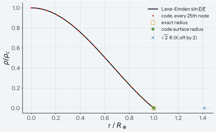
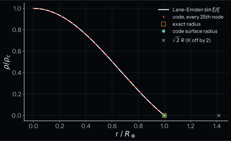
How to read the plot. The line is the Lane-Emden density \(\sin\xi/\xi\) against \(r/R_\oplus\) and gives context. The marks are the density that the test derives from the code pressure, over the central density, every 25th node, for 1 Earth mass. The test asserts the code surface radius (circle) against the exact radius \(R_\oplus\) (square) to a relative tolerance of \(10^{-4}\), too small to see. The cross is \(\sqrt{2}\,R_\oplus\), the radius with \(K\) off by a factor 2. A pass means that the circle sits in the square, far from the cross. The mass test and the mass-independence test are not drawn.

Grid and tolerance checks

Why this check exists. A finer grid or a tighter tolerance must not make the solution worse. The test fails in these cases:

• the mass error at \(N = 400\) reaches \(10^{-8}\);
• the pressure error at \(N = 400\) reaches \(10^{-6}\);
• the mass error at rtol \(= 10^{-12}\) reaches \(10^{-10}\);
• the mass error grows by more than a factor 1.5 from one grid or tolerance step to the next, but only above \(10^{-13}\), so at the measured errors of about \(2 \times 10^{-15}\) this rule does not act;
• a full-solver run does not converge, or the radii at \(N = 200\) and \(N = 400\) differ by 1 % or more.

A wrong factor in \(dM/dr\) or \(dg/dr\), or the wrong sign of \(dP/dr\), also makes the grid convergence test fail.

What it tests. The uniform-density sphere above on several grids and with several tolerances, and the full solver (the Picard outer solver and Brent's method) with the Analytic EOS at \(1\,M_\oplus\) on 3 grids.

• Grid convergence: the uniform sphere at \(N\) from 50 to 400 with rtol \(= 10^{-10}\). The mass error is \(2\) to \(3 \times 10^{-15}\) and the pressure error about \(4 \times 10^{-16}\) at every \(N\). The uniform-sphere solution is a cubic and a parabola in \(r\), which the integrator reproduces to round-off on every grid, so this case shows no convergence rate.
• Full solver: the planet radius is the same, \(0.96512\,R_\oplus\) (6114.5 km), at \(N = 100\), 200 and 400.
• Tolerance convergence: for rtol from \(10^{-6}\) to \(10^{-12}\) at \(N = 200\) the mass error stays between \(2\) and \(4 \times 10^{-15}\), with no trend: the error is at round-off level for every tolerance tested.

How we know the right answer. The closed-form solution of the uniform-density sphere gives the error. For the full solver, the radius on the finer grid (\(N = 400\)) is the reference for the radius at \(N = 200\) (self-consistency).

Why it matters. The default grid and tolerances of Zalmoxis must give a result that does not change when they are refined.

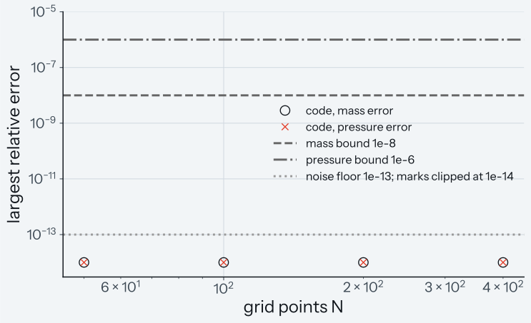
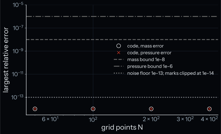
How to read the plot. Both axes are logarithmic. The circles are the asserted largest relative mass errors of the uniform sphere at \(N\) = 50 to 400. The crosses are its pressure errors from a second solve in the plot code; the pressure test asserts them. All are round-off, below \(3 \times 10^{-15}\), and are drawn at \(10^{-14}\) so that the plot is the same on every platform. The dashed and dash-dotted lines are the bounds at \(N = 400\): \(10^{-8}\) for the mass and \(10^{-6}\) for the pressure. The dotted line at \(10^{-13}\) is the floor above which an error may grow by at most a factor 1.5 per step. A pass means that the marks at \(N = 400\) lie below their bounds; the full-solver and tolerance tests are not drawn.

Known limit. The uniform sphere is solved to round-off at every \(N\), so the test shows no order of convergence. All errors are below \(10^{-13}\), so the factor 1.5 check is never applied.

JAX and numpy right-hand sides

Why this check exists. The optional JAX path (use_jax = True) evaluates the right-hand side of the structure equations in its own code, zalmoxis.jax_eos.rhs.coupled_odes_jax. If it differs from the numpy zalmoxis.structure_model.coupled_odes by more than the tolerance, a JAX run gives another structure than a numpy run, and these tests fail.

What it tests. The cases compare \(dM/dr\), \(dg/dr\) and \(dP/dr\) of the two codes on the same states.

Each table case draws random states with a fixed seed: \(r\) from \(10^5\) to \(6.4 \times 10^6\) m, \(M\) from 0 to \(1\, M_\oplus\), \(g\) from 0.5 to 25 m/s\(^2\) and \(P\) from \(10^6\) to \(3 \times 10^{11}\) Pa, with a PALEOS iron core and a PALEOS MgSiO\(_3\) mantle. A state counts when both codes return a nonzero right-hand side, and more than 100 states must count. JAX must never return a nonzero value where numpy returns zero.

The Tier column names the test group: unit tests need no table data, and integration tests need the PALEOS tables. The synthetic cases build small tables in memory, so they need no EOS files and run in the unit tier.

How we know the right answer. Two codes of the same equations must give the same \(dM/dr\), \(dg/dr\) and \(dP/dr\), so the numpy coupled_odes is the reference (a cross-code check).

Why it matters. Every run with use_jax = True integrates the structure with the JAX right-hand side, also when PROTEUS calls Zalmoxis on the JAX path.

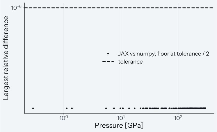
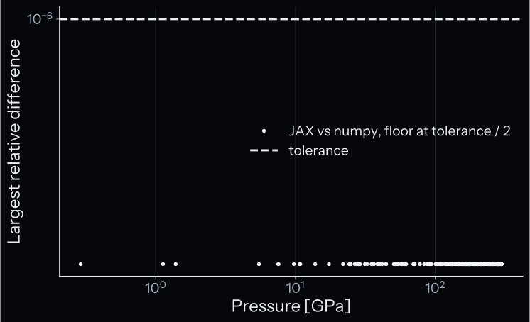
How to read the plot. Each marker is one compared state of the dry unified mantle case, with a PALEOS iron core and a unified PALEOS MgSiO\(_3\) mantle. It shows the largest relative difference of the 3 right-hand-side terms between coupled_odes_jax and coupled_odes, against the pressure of that state. The dashed line is the tolerance, 1e-6. A difference below half the tolerance is drawn at that floor, because its exact value changes between platforms. On the machine that made the plot, the largest difference is 1.4e-7. A pass means that every marker lies below the dashed line.

Known limit. In at most 4 of 200 states numpy returns a nonzero value where JAX returns zero: the numpy tables fall back to the nearest table cell outside their range, and the JAX path has no such fallback.

Surface boundary condition of the pressure solve

Why this check exists. Brent's method can return a central pressure for which the integration stops below the surface, and the solve must then refine that root. If the refinement does not run, or keeps the padded root, the profile ends with a pressure of 0 at the outer radius instead of the surface pressure.

What it tests. The central pressure \(P_c\) is the root of the residual \(f(P_c) = P(R) - P_t\). Here \(P(R)\) is the pressure at the outer radius \(R\), and \(P_t\) is the target surface pressure, 1 atm here.

A trial \(P_c\) whose integration stops before the outer radius gives \(f = -P_t\), and the remaining points get zero pressure: this is a padded profile. Brent's method stops when its bracket is narrower than xtol \(= 10^6\) Pa, and it can then return such a padded root. The solve then refines the root (padded accepts).

The test uses an analytic residual that needs no structure solve. Below a central pressure \(x_0\) the integration stops; above it, \(P(R)\) rises from \(0.95\,P_t\) at a slope \(dP(R)/dP_c\) of 0.47. The Brent root of the first solve is then padded, and the refined root must reach the outer radius and miss \(P_t\) by at most \(0.1 P_t\).

A second test checks the same rule with real structure solves. It uses the Analytic 1 Earth-mass planet with the Newton outer solver at relative_tolerance \(10^{-9}\), and shifts the planet mass by a relative amount of 0 and \(\pm 10^{-9}\) until a pressure solve has a padded Brent root. The refined root must then miss \(P_t\) by at most \(0.1 P_t\). The accepted profile must not be padded, and it must miss \(P_t\) by at most \(P_t\).

How we know the right answer. The boundary condition \(P(R) = P_t\) gives the right answer. A profile that reaches the outer radius with \(P(R)\) close to \(P_t\) meets it. A padded profile has \(P(R) = 0\), so it misses by the full \(P_t\).

Why it matters. The accepted profile is the structure that Zalmoxis returns, for example to PROTEUS. Its outer point must have the surface pressure that the run asks for, not a padded pressure of 0.

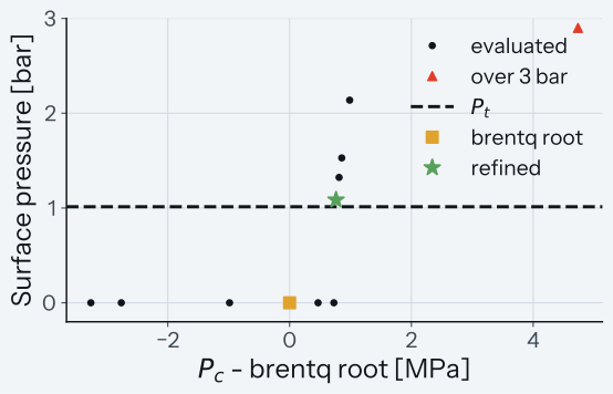
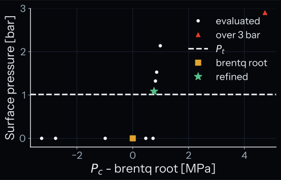
How to read the plot. The x-axis is the central pressure relative to the Brent root of the first solve, in MPa, and the y-axis is the surface pressure \(P(R)\) in bar. Each circle is one evaluated central pressure. The square is the padded Brent root of the first solve (\(P(R) = 0\)), and the star is the refined root, which reaches the outer radius. Evaluations above 3 bar are drawn as triangles at the top of the axis, and the dashed line is \(P_t\) = 1 atm. A pass means that the star lies within \(0.1 P_t\) of the dashed line.

Known limit. Whether a real solve pads depends on round-off, so the test with real structure solves has no plot.

Surface boundary condition in every Newton setup

Why this check exists. The refinement must also work on the real equations of state of a planet, not only on an analytic residual. If it fails there, the accepted profile of a Newton run ends padded, or it misses the surface pressure by more than \(P_t\).

What it tests. The test runs the 6 Newton setups: the Analytic EOS (equation of state) at 1 Earth mass, PALEOS at 1, 5 and 10 Earth masses, and PALEOS on the JAX path with \(T(r)\) from a numpy Picard solve at 1 and 3 Earth masses.

Every setup must accept on the Newton tolerance. Every reached profile must miss \(P_t\) by at most \(P_t\), and no profile may have a padded node, except on the JAX path at 1 Earth mass.

On that path \(P(R)\) varies irregularly from one trial central pressure to the next near the surface stop, where the integration ends before the outer radius, and the accepted profile can be padded. The case then requires one of 2 things: the reached end of the first sign pair of that pressure solve misses \(P_t\) by more than \(P_t\), or the solve has no sign pair.

How we know the right answer. As in the case above, the boundary condition \(P(R) = P_t\) gives the right answer.

Why it matters. The Newton outer solver at relative_tolerance \(10^{-9}\) is the outer solver that PROTEUS uses by default. These setups run it on the PALEOS tables from 1 to 10 Earth masses, on the numpy and the JAX path.

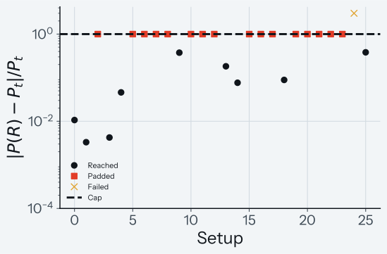
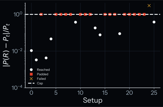
How to read the plot. The x-axis is the number of the setup, for 26 setups built from input/default.toml and numbered from 0 to 25. The y-axis is \(\lvert P(R) - P_t \rvert / P_t\) of the accepted profile, on a log scale. Circles are reached profiles, squares are padded profiles (at 1, since \(P(R) = 0\)), and a cross above the cap marks a setup without an accepted profile. The dashed line is the cap of \(P_t\). Setups 4, 9, 10, 13, 14 and 25 use the Newton outer solver at relative_tolerance \(10^{-9}\), and the test asserts only these 6; the other 20 setups are shown for comparison; padded accepts lists every setup. A pass means that every Newton setup is a circle at or below the dashed line. Only setup 10 may be a square, and only under the rule of the JAX path above.

Known limit. The miss of a reached profile depends on round-off, so another platform gives other values. Over planet-mass changes of \(k \times 10^{-13}\) (\(k\) = 1 to 5), the PALEOS 1 Earth-mass Newton setup misses by 0.008 to 0.87 \(P_t\). The test skips when the PALEOS tables are not under data/.

Reproducing the results

The tests draw the plots of these cases. This command writes them again to docs/assets/validation/:

pytest -o "addopts=" tests/test_first_principles.py tests/test_polytrope_verification.py --validation-plots

Without --validation-plots the tests write nothing: each compares the data of its plot with the committed pair, and a missing or stale file fails the test.