Parameter grids
To sweep over any combination of parameters, use the grid runner with a TOML specification file:
python -m tools.grids.run_grid <grid.toml> -j <workers>
The -j flag sets the number of parallel workers (default: 1, serial execution).
Grid TOML format
A grid TOML file has three sections:
[base]
config = "input/default.toml"  # base config (relative to ZALMOXIS_ROOT)

[sweep]
# Each key is a parameter name, each value is a list to sweep over.
# The runner generates the Cartesian product of all sweep parameters.
planet_mass = [0.5, 1.0, 3.0, 5.0, 10.0]
surface_temperature = [1000, 2000, 3000]

[output]
dir = "output/grid_results"        # output directory (relative to ZALMOXIS_ROOT)
save_profiles = true               # optional (default false); see Output section
The available sweep parameter names and their mapping to TOML config sections are:
| Sweep parameter | Config section | Config key |
|---|---|---|
planet_mass |
[InputParameter] |
planet_mass |
core_mass_fraction |
[AssumptionsAndInitialGuesses] |
core_mass_fraction |
mantle_mass_fraction |
[AssumptionsAndInitialGuesses] |
mantle_mass_fraction |
temperature_mode |
[AssumptionsAndInitialGuesses] |
temperature_mode |
surface_temperature |
[AssumptionsAndInitialGuesses] |
surface_temperature |
center_temperature |
[AssumptionsAndInitialGuesses] |
center_temperature |
core |
[EOS] |
core |
mantle |
[EOS] |
mantle |
ice_layer |
[EOS] |
ice_layer |
condensed_rho_min |
[EOS] |
condensed_rho_min |
condensed_rho_scale |
[EOS] |
condensed_rho_scale |
binodal_T_scale |
[EOS] |
binodal_T_scale |
mushy_zone_factor |
[EOS] |
mushy_zone_factor |
rock_solidus |
[EOS] |
rock_solidus |
rock_liquidus |
[EOS] |
rock_liquidus |
num_layers |
[Calculations] |
num_layers |
target_surface_pressure |
[PressureAdjustment] |
target_surface_pressure |
Example: mass-radius curve
Sweep planet mass to build a mass-radius relation for rocky planets (file: input/grids/mass_radius.toml):
[base]
config = "input/default.toml"

[sweep]
planet_mass = [0.5, 1.0, 2.0, 3.0, 5.0, 7.0, 10.0]

[output]
dir = "output/grid_mass_radius"
Run with 2 workers:
python -m tools.grids.run_grid input/grids/mass_radius.toml -j 2
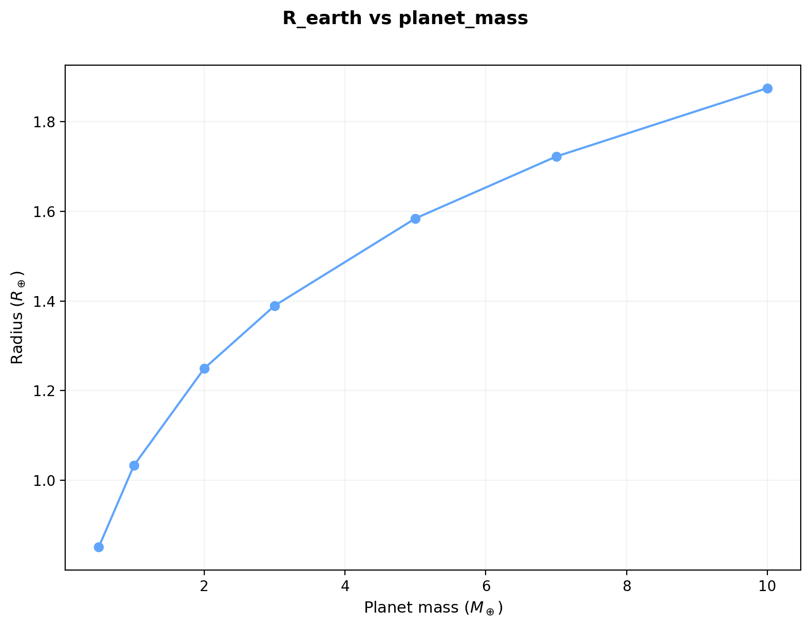
The resulting mass-radius relation for a PALEOS iron core + MgSiO3 mantle planet (32.5% core mass fraction, adiabatic temperature at \(T_s\) = 3000 K):
Example: H\(_2\) mixing grid
Sweep planet mass, mantle composition, and surface temperature to explore the effect of dissolved hydrogen on planet radius (file: input/grids/h2_mixing.toml):
[base]
config = "input/default.toml"

[sweep]
planet_mass = [1.0, 3.0, 5.0, 10.0]
mantle = ["PALEOS:MgSiO3", "PALEOS:MgSiO3:0.97+Chabrier:H:0.03", "PALEOS:MgSiO3:0.90+Chabrier:H:0.10"]
surface_temperature = [2000, 3000]

[output]
dir = "output/grid_h2_mixing"
This produces 4 x 3 x 2 = 24 models. Plotting with --single-panel shows how dissolved hydrogen inflates the radius at fixed mass:
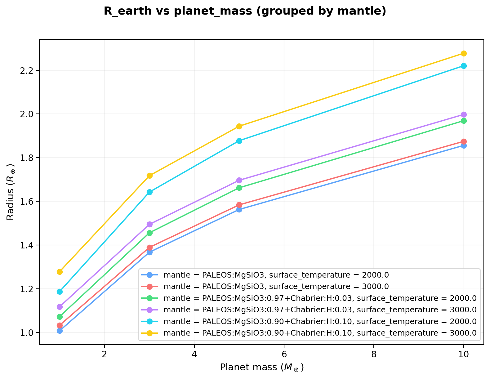
At higher H\(_2\) mass fractions, the lower mean density of the mixed mantle leads to larger radii, with the effect increasing at higher masses where the mantle constitutes a larger fraction of the planet volume.
Example: H\(_2\)O mixing grid
Sweep planet mass and mantle water content to explore the effect of water on planet radius (file: input/grids/h2o_mixing.toml):
[base]
config = "input/default.toml"

[sweep]
planet_mass = [1.0, 3.0, 5.0, 10.0]
mantle = ["PALEOS:MgSiO3", "PALEOS:MgSiO3:0.90+PALEOS:H2O:0.10", "PALEOS:MgSiO3:0.50+PALEOS:H2O:0.50"]
surface_temperature = [2000, 3000]

[output]
dir = "output/grid_h2o_mixing"
This produces 4 x 3 x 2 = 24 models. Plotting with --single-panel shows the radius increase from water in the mantle:

Example: varying temperature and planet mass
Sweep surface temperature and planet mass to explore thermal expansion effects on radius (file: input/grids/mass_temperature.toml):
[base]
config = "input/default.toml"

[sweep]
planet_mass = [0.5, 1.0, 3.0, 5.0, 10.0]
surface_temperature = [1000, 2000, 3000, 4000]

[output]
dir = "output/grid_mass_temperature"
This produces 5 x 4 = 20 models. Plotting with --single-panel overlays all temperature curves on one panel:
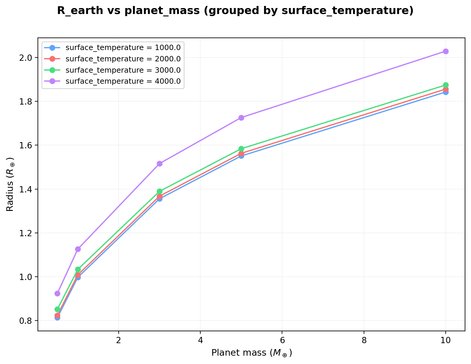
Higher surface temperatures lead to larger radii through thermal expansion. The effect is modest between 1000 and 3000 K but becomes significant at 4000 K, particularly at lower masses where self-compression is weaker.
Output
Each grid run produces:
grid_summary.csv: One row per model with columns for all sweep parameters, calculated radius (R_earth), mass (M_earth), convergence flags, wall time, and any error messages.- Per-run JSON files: Individual
<label>.jsonfiles with the same summary information, named by the parameter combination. -
Per-run profile files (optional,
[output].save_profiles = true, defaultfalse):<label>.csvfiles containing the full radial structure of each grid point. Each CSV has an eight-column body and a# key: valuecomment header. The body contains six numeric SI columns (radius_m,density_kg_m3,gravity_m_s2,pressure_Pa,temperature_K,mass_enclosed_kg) plus two string columns labelling the dominant chemistry and its phase per radial shell:main_component: the dominant (highest mass-fraction) chemistry of the layer the shell sits in (Fe,MgSiO3,H2O,H2, ...). For multi-component layers (e.g.mantle = "PALEOS:MgSiO3:0.85+PALEOS:H2O:0.15") only the dominant component is reported.phase: the phase of that component at the shell's (P, T). One ofsolid,liquid,gas,supercritical,mixed(mushy zone for 2-phase silicate EOS), orunknown. Phase is read directly from the unified PALEOS table's per-cell phase column forPALEOS:iron,PALEOS:MgSiO3,PALEOS:H2O; from the configured solidus & liquidus forPALEOS-2phase:*,WolfBower2018:*,RTPress100TPa:*; hardcoded tosupercriticalforChabrier:H(always above the H2 critical point at planetary interior conditions); andsolidforSeager2007:*(300 K static lookup tables for solid-phase Fe/silicate/water).
The comment header carries the scalar mass diagnostics (
cmb_mass,core_mantle_mass), theconvergedflag, the run label, and the per-layer EOS and melting-curve identifiers (core_eos,mantle_eos,ice_layer_eos,rock_solidus_id,rock_liquidus_id).CSVs are written for non-converged grid points too (useful for debugging), but the last row of
radius_mandmass_enclosed_kgin those cases is the last Picard iterate, not the planet's converged structure, anddensity_kg_m3can contain NaN or zero in failed or padded shells. Filter onconverged == Truebefore plotting.
Plotting is always disabled during grid runs for speed. To generate the per-planet matplotlib plots for a specific parameter combination, run that case individually (python -m zalmoxis -c <cfg>.toml) with plots_enabled = true.
Loading saved profiles
Each <label>.csv opens directly in any spreadsheet or text editor; the # key: value header lines are ignored by pandas.read_csv(..., comment='#') and by numpy.loadtxt(..., comments='#'). To plot pressure vs. radius for a grid point labelled planet_mass=3.0:
import pandas as pd
import matplotlib.pyplot as plt

df = pd.read_csv('output/grid_mass_radius/planet_mass=3.0.csv', comment='#')
plt.plot(df['radius_m'] / 1e3, df['pressure_Pa'] / 1e9)  # km, GPa
plt.xlabel('Radius [km]')
plt.ylabel('Pressure [GPa]')
plt.show()
The converged flag and other metadata sit in the comment header; the bundled tools.plots._grid_io.load_profile(grid_dir, label) helper parses both halves into a single dict if you need programmatic access.
Typical file sizes are a few tens of kB per grid point (uncompressed text), so 1000-point sweeps stay under a few hundred MB. Set save_profiles = false (or omit the key) if you only need the summary CSV.
Plotting grid results
Use plot_grid to visualize the results from a grid run:
python -m tools.grids.plot_grid output/grid_mass_radius
This reads the grid_summary.csv in the given directory and produces a mass-radius diagram by default. You can also pass the CSV path directly:
python -m tools.grids.plot_grid output/grid_mass_radius/grid_summary.csv
Choosing axes
Any column in the CSV can be used as the x- or y-axis:
python -m tools.grids.plot_grid output/grid_results -x surface_temperature -y R_earth
Available columns include all sweep parameters (planet_mass, surface_temperature, core_mass_fraction, etc.) and computed outputs (R_earth, M_earth, time_s).
Multi-parameter grids
When the grid sweeps two or more parameters, the plotter automatically groups by the second sweep parameter and creates one subplot per group value:
# 2D grid (mass x surface_temperature): one subplot per surface_temperature
python -m tools.grids.plot_grid output/grid_results
To override which parameter is used for grouping:
python -m tools.grids.plot_grid output/grid_results -g mantle
To put all groups on a single panel with a color-coded legend instead of subplots:
python -m tools.grids.plot_grid output/grid_results --single-panel
Unconverged runs
Runs that did not converge are shown as X-shaped markers (with a separate legend entry), so they are visible but distinct from converged results. Runs that failed entirely (no radius computed) are silently skipped.
Plot output
By default, the figure is saved in the same directory as the CSV with a descriptive filename (e.g., grid_R_earth_vs_planet_mass.png). To specify a different output path:
python -m tools.grids.plot_grid output/grid_results -o my_plot.png
Python API
The plotting function can also be called directly from Python (e.g., in a Jupyter notebook or IDE):
from tools.grids.plot_grid import plot_grid_summary

# Default mass-radius plot
plot_grid_summary("output/grid_mass_radius")

# Custom axes, single panel
plot_grid_summary(
    "output/grid_results",
    x="surface_temperature",
    y="R_earth",
    group_by="mantle",
    single_panel=True,
    output="my_plot.png",
)
Full CLI reference
python -m tools.grids.plot_grid <path> [-x COLUMN] [-y COLUMN] [-g PARAM]
                               [--single-panel] [-o FILE] [--dpi N]
| Flag | Default | Description |
|---|---|---|
path |
(required) | Grid output directory or grid_summary.csv path |
-x |
planet_mass |
Column for the x-axis |
-y |
R_earth |
Column for the y-axis |
-g |
auto | Sweep parameter to group by |
--single-panel |
off | All groups on one panel |
-o |
auto | Output file path |
--dpi |
200 | Figure resolution |
Plotting saved radial profiles
When the grid was run with [output].save_profiles = true, three companion tools read the per-grid-point .csv profiles and produce figures that are complementary to the scalar M-R plots from plot_grid.
plot_grid_profiles: radial-profile overlay (2x2)
Overlays density, pressure, temperature, and gravity vs. radius across every converged grid point, coloured by the primary sweep parameter. The natural companion to the plot_grid M-R diagram for answering "how does the interior change across the sweep?".
python -m tools.plots.plot_grid_profiles output/grid_mass_radius
python -m tools.plots.plot_grid_profiles output/grid_mass_radius -o profiles.pdf
python -m tools.plots.plot_grid_profiles output/grid_mass_radius --colour-by surface_temperature --log-pressure
Default output: <grid_dir>/profiles_vs_radius.pdf. Non-converged grid points and points without a saved profile CSV are skipped with a note on stdout. Full CLI:
| Flag | Default | Description |
|---|---|---|
path |
(required) | Grid output directory or grid_summary.csv path |
-o, --output |
profiles_vs_radius.pdf |
Output file (extension selects format) |
--colour-by |
first numeric sweep parameter | Sweep parameter used for line colour |
--log-pressure |
off | Logarithmic pressure y-axis |
--dpi |
200 | Raster DPI (ignored for vector formats) |
Python API:
from tools.plots.plot_grid_profiles import plot_grid_profiles

plot_grid_profiles("output/grid_mass_radius")  # default: profiles_vs_radius.pdf
plot_grid_profiles("output/grid_h2_mixing", colour_by="surface_temperature")
plot_grid_pt: interior pressure-temperature trajectories
Plots the full interior (P, T) trajectory of every converged grid point as one line, coloured by the primary sweep parameter. Pressure is log-scaled by default. The core-mantle boundary of each trajectory is marked with a black-edged dot. The tool reads EOS and melting-curve metadata from each profile CSV's comment header and overlays mantle solidus and liquidus curves only when the solver actually used external curves (WolfBower2018:MgSiO3, RTPress100TPa:MgSiO3, PALEOS-2phase:MgSiO3). For unified PALEOS tables (e.g., PALEOS:MgSiO3), where the phase boundary is embedded in the EOS table itself, the overlay is suppressed by default and a short note is printed on the figure explaining why. Use --solidus / --liquidus to force a specific overlay for visual comparison.
Useful for diagnosing which EOS phase regimes the sweep traverses and for sanity-checking that interior conditions stay inside the pressure/temperature range covered by the selected tables.
python -m tools.plots.plot_grid_pt output/grid_mass_radius
python -m tools.plots.plot_grid_pt output/grid_mass_radius -o pt.pdf
python -m tools.plots.plot_grid_pt output/grid_mass_radius --linear-pressure
python -m tools.plots.plot_grid_pt output/grid_mass_radius \
    --solidus Stixrude14-solidus --liquidus Stixrude14-liquidus
python -m tools.plots.plot_grid_pt output/grid_mass_radius --no-melting-curves
Default output: <grid_dir>/pt_trajectories.pdf. Full CLI:
| Flag | Default | Description |
|---|---|---|
path |
(required) | Grid output directory or grid_summary.csv path |
-o, --output |
pt_trajectories.pdf |
Output file (extension selects format) |
--colour-by |
first numeric sweep parameter | Sweep parameter used for line colour |
--linear-pressure |
off | Linear pressure y-axis (default is log) |
--solidus |
auto-detect from CSV header | Force a solidus curve id (zalmoxis.melting_curves) |
--liquidus |
auto-detect from CSV header | Force a liquidus curve id |
--no-melting-curves |
off | Disable the solidus/liquidus overlay entirely |
--dpi |
200 | Raster DPI (ignored for vector formats) |
The metadata fields the tool reads (mantle_eos, rock_solidus_id, rock_liquidus_id) are written into the CSV comment header by run_grid when save_profiles = true. If a grid was run with an older format that omits this metadata, the overlay is suppressed with a note pointing to the fix (re-run the grid).
Python API:
from tools.plots.plot_grid_pt import plot_grid_pt

plot_grid_pt("output/grid_mass_radius")  # default: pt_trajectories.pdf
plot_grid_pt(
    "output/grid_mass_radius",
    solidus="Stixrude14-solidus",
    liquidus="Stixrude14-liquidus",
)
plot_grid_composition: layer composition bars
Draws two horizontal stacked-bar panels: core / mantle / ice fractions by mass on the left, and by radius on the right, one bar per converged grid point. Core and mantle are always shown; the ice / envelope segment appears only for 3-layer runs (or when the mantle mass fraction plus ice layer add up to less than the total). Bars are sorted numerically by the labelling sweep parameter so the ordering is intuitive.
Useful for seeing at a glance how a composition sweep reshapes the layering (h2_mixing, h2o_mixing grids) or how self-compression shifts the core radius fraction at fixed composition (mass_radius, mass_temperature grids).
python -m tools.plots.plot_grid_composition output/grid_mass_radius
python -m tools.plots.plot_grid_composition output/grid_h2_mixing --label-by mantle
python -m tools.plots.plot_grid_composition output/grid_mass_radius -o composition.pdf
Default output: <grid_dir>/composition.pdf. Full CLI:
| Flag | Default | Description |
|---|---|---|
path |
(required) | Grid output directory or grid_summary.csv path |
-o, --output |
composition.pdf |
Output file (extension selects format) |
--label-by |
first sweep parameter | Sweep parameter whose value labels each bar |
--dpi |
200 | Raster DPI (ignored for vector formats) |
Python API:
from tools.plots.plot_grid_composition import plot_grid_composition

plot_grid_composition("output/grid_mass_radius")
plot_grid_composition("output/grid_h2_mixing", label_by="mantle")