Usage

Quick start

Run the default configuration (1 Earth-mass planet with a PALEOS iron core and MgSiO3 mantle):

python -m zalmoxis -c input/default.toml

Output files appear in output_files/. The PALEOS data files must be downloaded first (see installation).

What happens when you run Zalmoxis

Zalmoxis computes the internal structure of a planet. Given a total mass and composition (which layers the planet has, and what each layer is made of), it finds the radial profiles of pressure, density, gravity, and temperature from the center to the surface. The result is a self-consistent model of the planet's interior: how big it is, where the core-mantle boundary sits, and how conditions change with depth.

For the mathematical details of how the solver works, see the process flow explanation.

Modifying the configuration

All input parameters live in a single TOML file. To change the planet mass, for example, open input/default.toml and edit the [InputParameter] section.

Before:

[InputParameter]
planet_mass = 1.0  # in Earth masses

After (5 Earth-mass super-Earth):

[InputParameter]
planet_mass = 5.0  # in Earth masses

Then re-run:

python -m zalmoxis -c input/default.toml

For the full list of parameters (EOS selection, temperature modes, solver settings, output options), see the configuration reference.

Output files

All output files are written to the output_files/ directory (created automatically on first run). The directory structure looks like:

output_files/
├── planet_profile.txt            # radial profiles (single run)
├── planet_profile5.0.txt         # radial profiles (batch run, mass in filename)
├── calculated_planet_mass_radius.txt  # summary: mass and radius per run
├── planet_profile.png            # 6-panel structure plot (if plots_enabled)
├── grid_results/                 # grid runner output (if using run_grid)
│   ├── grid_summary.csv
│   └── *.json
└── pressure_profiles.txt         # iteration diagnostics (if enabled)

Profile files

When data_enabled = true (the default), the solver writes radial profiles as tab-separated text:

• planet_profile.txt: Full radial profile for a single-mass run.
• planet_profile{mass}.txt: Same format, with the planet mass (in Earth masses) appended. Produced by batch runs to distinguish between different masses.

The columns are:

The first row is the center (r = 0) and the last row is the surface. Shells beyond the planet surface (where the ODE terminal event fired) are padded with zeros.

Summary file

• calculated_planet_mass_radius.txt: Two-column summary (calculated mass in kg, calculated radius in m). Each row corresponds to one completed simulation. Appended across successive runs, so multiple runs accumulate in one file.

Iteration profiles (optional)

When iteration_profiles_enabled = true in the [Output] section:

• pressure_profiles.txt: Pressure vs. radius for every iteration of the pressure adjustment loop.
• density_profiles.txt: Density vs. radius for every iteration.

These files are useful for diagnosing convergence behavior. They grow large quickly and are overwritten at the start of each new run. Leave disabled for production runs.

Plots (optional)

When plots_enabled = true in the [Output] section, Zalmoxis automatically generates profile plots after each run. To enable:

[Output]
plots_enabled = true

This produces a six-panel figure showing the radial profiles of density, pressure, temperature, gravity, phase state, and mass enclosed:

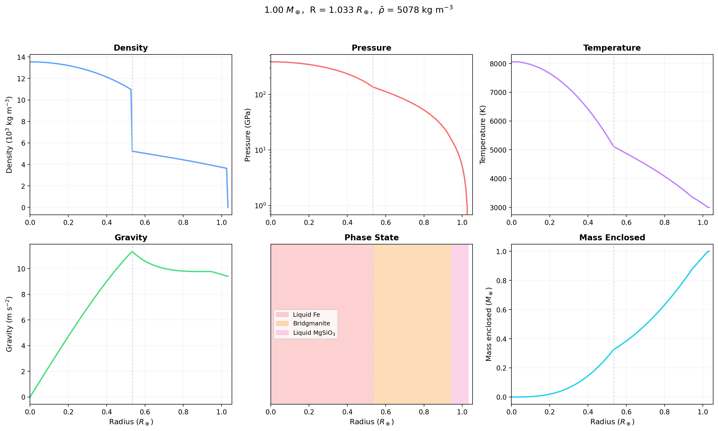
Example: 1 \(M_\oplus\) planet with a PALEOS iron core and MgSiO\(_3\) mantle at \(T_s\) = 3000 K (adiabatic mode). The dashed vertical line marks the core-mantle boundary (CMB).

• Density (top left): drops from ~14,000 kg/m\(^3\) at the center (iron core) to ~3,000 kg/m\(^3\) at the surface (silicate mantle). The sharp step at the CMB reflects the iron-to-silicate transition.
• Pressure (top center): decreases monotonically from ~350 GPa at the center to 1 atm at the surface, on a logarithmic scale.
• Temperature (top right): follows the adiabatic gradient from 3000 K at the surface to ~8000 K at the center. The steeper gradient in the iron core reflects iron's different \(\nabla_{\mathrm{ad}}\).
• Gravity (bottom left): rises through the core (as enclosed mass grows faster than \(r^2\)), peaks near the CMB at ~10 m/s\(^2\), and stays roughly constant through the mantle.
• Phase state (bottom center): colored bars showing the thermodynamically stable phase at each depth, read from the PALEOS table's phase column. Liquid iron in the core (at 3000 K surface temperature), bridgmanite (solid MgSiO\(_3\)) in the mantle, with a thin liquid layer near the surface.
• Mass enclosed (bottom right): enclosed mass as a function of radius. The CMB is visible as the kink where the slope changes from the dense core to the lighter mantle.

Parameter grids

To sweep over combinations of parameters and plot the results, see the parameter grids guide.