Core module verification
This page checks the core_module core boundary condition (core_bc.md) and the aragog.core model behind it against analytic results, published values, an independent core evolution code and coupled runs. Each section states the physics a check tests, the reference and where it comes from, the value aragog gives, a figure and what it shows, the limits of the check where it has any, and the tests that pin it. A check shows that the code solves the stated equations to the stated accuracy; whether the equations describe a real core is a separate question, which the literature comparisons in sections 5 to 8 and the limits stated with each check address.
Every number on this page and every figure is produced by tools/verification/run_core_verification.py, which writes the figures to docs/figures/vv/ and the numbers to docs/figures/vv/core_verification_values.json; tests/test_core_verification_page.py checks each number on the page against that file. The script needs the SPIDER-format EOS tables (ARAGOG_TEST_EOS_DIR) for sections 9 and 12 and the optional verification dependencies for the figure style, and runs in about eight minutes on one core. Sections 9 and 12 and the solver tests use the aragog test tables that CI uses, spider_eos_test_data.tar.gz of release test-data-v1 (sha256 e3842bc494969571428d7f978d8f70972d40a3bc5d6ac2c09f6a96808f4079fb), 500 pressures from 0 to 150 GPa by 200 entropies; their numbers hold for these tables. Other tables give other values; section 12 compares two sets of 1350 pressures by 280 entropies that reach 650 GPa. Two kinds of number come from separate measurements and say so where they appear: the closures of the stratified call heated from above (section 13), held by its smoke test, and the expansivity differences on those two sets. Nimmo (2015) is chapter 8.02 of the Treatise on Geophysics wherever chapter 9.08 is not named.
1. Gaussian core structure
What is tested. The core density is a Gaussian in radius,
with \(\rho_\mathrm{cen}\) the central density and \(L\) the length scale, and the adiabat solves
with \(\alpha\) the thermal expansivity, \(g\) the gravity and \(c_p\) the heat capacity. By default it uses the exact gravity (adiabat_mode = "exact"),
with \(\psi\) the gravitational potential, zero at the CMB, on the Gauss-Legendre panel of the pressure. The closed form (adiabat_mode = "small_radius")
(Labrosse et al. 2001, eqs. 7 and 11, the adiabat to the same order in radius as their density and gravity, eq. 8) holds for gravity linear in \(r\); Nimmo (2015) and thermal_history use it, so sections 5, 6, 7, 10 and 13 do too. Mass and gravity are closed-form integrals of the density; the pressure is the hydrostatic integral of \(\rho g\) from the CMB inward, by 32-point Gauss-Legendre quadrature (pressure_mode = "quadrature"), or the third-order expansion in \(r/L\) that Labrosse et al. (2001, eq. 8) use for gravity (pressure_mode = "labrosse").
Reference. The checks run on the Earth-like test core (\(\rho_\mathrm{cen} = 12500\) kg m\(^{-3}\), \(L = 7200\) km, \(r_\mathrm{cmb} = 3480\) km). The references are an independent adaptive quadrature of the density, the linear limit of gravity near the centre, \(4\pi G \rho_\mathrm{cen} r/3\), and hydrostatic balance, \(dP/dr = -\rho g\).
Result. The core has a mass of 1.92e+24 kg, a CMB density of 9896 kg m\(^{-3}\) and a central pressure of 356.8 GPa. On this test core, \(T_\mathrm{cen}/T_\mathrm{cmb}\) is 1.374 with the exact gravity and 1.405 in the closed form.
| Check | Relative difference |
|---|---|
| Closed-form enclosed mass and gravity against the adaptive quadrature | 3.6e-13 |
| Gravity near the centre against the linear limit | 2.2e-16 |
| Hydrostatic balance of the pressure | 2.5e-08, the error of the 50 m central difference used to test it |
| Third-order pressure against the quadrature | up to 3.0e-03, the truncation of the expansion |
Both pressures meet the CMB anchor exactly.
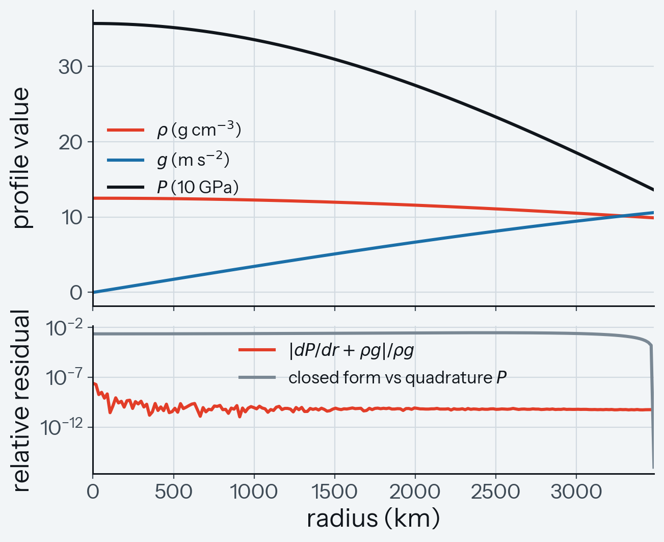
Figure 1. Gaussian core structure of the Earth-like test core. (a) Density, gravity and pressure against radius. (b) Relative residual of hydrostatic balance \(|dP/dr + \rho g|/\rho g\) for the quadrature pressure, and the relative difference between the third-order and the quadrature pressure; both panels share the radius axis.
What the figure shows. In (b) the residual of hydrostatic balance stays at or below the value of the result at every radius, and the difference of the third-order pressure is flat at its truncation level and falls to zero at the CMB, where both pressures are anchored. A pressure with a wrong slope would lift the residual by orders of magnitude. The pressure sets where the melting curve is evaluated, so the inner-core radius of a core_module run depends on it.
Pinned by tests/test_core_profiles.py::test_density_positive_monotone_and_mass_matches_quadrature, ::test_gravity_centre_limit_and_shell_integral and ::test_pressure_hydrostatic_balance_and_anchor.
2. Energy identities of the core budget
What is tested. The core cools at
where the effective capacity \(\tilde C\) adds the secular term, the latent heat of inner-core growth and the gravitational energy of the light elements it rejects, \(Q_\mathrm{cmb}\) is the CMB heat flow and \(Q_\mathrm{radio}\) the radiogenic power. The heat content \(H(T)\) is defined so that
the solver books the core heat change from it, so this identity is what ties the core ledger to the CMB heat. Inner-core growth starts at the onset temperature \(T_\mathrm{on}\), where the adiabat first touches the melting curve at the centre, and ends at freeze-out \(T_\mathrm{fr}\), where the whole core has crystallised and the latent and gravitational terms vanish.
Reference. The reference is the integral of \(\tilde C\) by a trapezoid rule on 40001 points, on the test core of section 1 with the iron-alloy curve. The comparison covers 150 K on either side of the growth band, the CMB temperatures from the onset to the freeze-out, where the inner core grows.
Result. For the iron-alloy curve on the test core, onset is at 4146.7 K and freeze-out at 3688.9 K. The heat-content difference matches the integral of \(\tilde C\) to 6.6e-07 of the total; the residual above the onset is the trapezoid error of that reference at the square-root cusp of the latent term, not an error of \(H\). At freeze-out the capacity drops by a factor of 3.143 for the Nimmo (2015) quadratic curve and by 50.5 % for the iron-alloy curve, without the gravitational term.
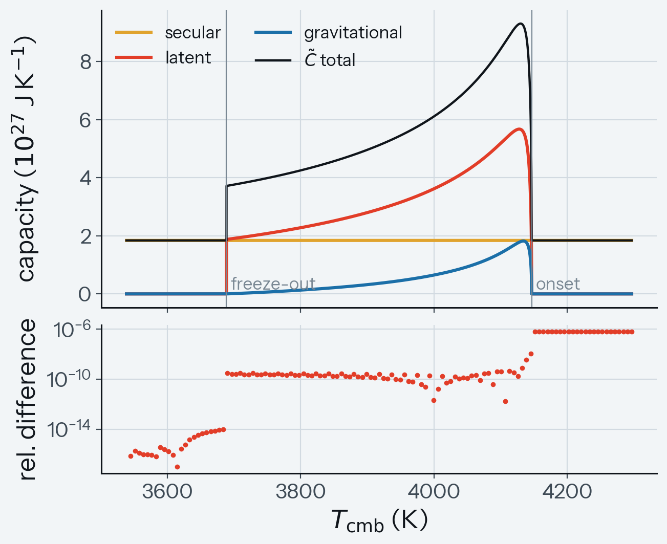
Figure 2. Effective heat capacity of the core across inner-core growth. (a) Secular, latent and gravitational capacities and their sum against CMB temperature, with the onset and freeze-out marked. (b) Relative difference between the heat-content difference and the integral of the total capacity at 120 temperatures, normalised by the total.
What the figure shows. In (a) the latent and gravitational capacities are zero outside the growth band, rise steeply below the onset, and the latent one ends in a step at the freeze-out, where the total falls back to the secular capacity. In (b) the difference stays within the value of the result at every temperature. A heat content without the latent term would differ inside the band by a share of order one. The core ledger of a core_module run closes only if this identity holds.
Pinned by tests/test_core_budget.py::test_heat_content_difference_is_the_capacity_integral, ::test_latent_and_gravitational_energy_conservation (latent and gravitational capacities integrate to the geometric latent heat and gravitational energy to below 1e-6) and ::test_freeze_out_capacity_jump.
3. CMB boundary-layer flux
What is tested. For a core hotter than the mantle side of the CMB, the CMB heat flux is
where \(\Delta T = T_\mathrm{core} - T_m\), \(\Delta r_{1/2}\) is the distance to the bottom mantle cell and \(\delta\) is the boundary-layer thickness at the critical Rayleigh number (Foley & Driscoll 2016, eq. 20 and the text below it; Thiriet et al. 2019, eqs. 13 and 14). On the convective branch \(q \propto \Delta T^{4/3}\); a core colder than the mantle gains heat by conduction across the half cell only, so the flux always has the sign of \(\Delta T\).
Reference. The law is evaluated for a bottom cell with constant properties, over a liquid and a solid base:
| Property | Value |
|---|---|
| Conductivity \(k\) | 4 W m\(^{-1}\) K\(^{-1}\) |
| Density \(\rho\) | 4000 kg m\(^{-3}\) |
| Heat capacity \(c_p\) | 1000 J kg\(^{-1}\) K\(^{-1}\) |
| Expansivity \(\alpha\) | \(3\times10^{-5}\) K\(^{-1}\) |
| Gravity \(g\) | 10 m s\(^{-2}\) |
| Half cell \(\Delta r_{1/2}\) | 10 km |
| Viscosity \(\eta\) of the liquid base | 0.1 Pa s |
| Viscosity \(\eta\) of the solid base | \(10^{21}\) Pa s |
The default \(Ra_\mathrm{crit} = 450\) is the critical value Thiriet et al. (2019, Table 2) use for the upper boundary layer of their mantle; for the lower boundary layer they scale it with the internal Rayleigh number (their eq. 16), so here it is a parameter, ra_crit_cmb.
Result. The convective branch has the slope 1.333 in log-log and \(Ra_\mathrm{crit} = 1800\) lowers the flux by the factor 0.630 \(= (450/1800)^{1/3}\). At a 100 K contrast the flux is 5.55e+04 W m\(^{-2}\) over the liquid base and 0.04 W m\(^{-2}\) over a solid base, where conduction across the half cell sets it; a colder core conducts at the same rate over either base, to 4.2e-15.
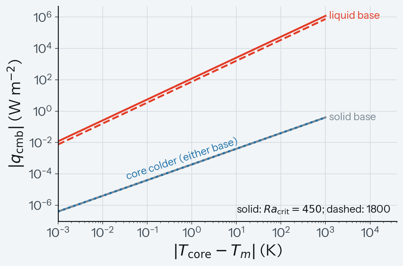
Figure 3. Magnitude of the CMB heat flux against the core-mantle temperature contrast, for a liquid and a solid bottom cell with the properties of section 3, at \(Ra_\mathrm{crit} = 450\) (solid) and 1800 (dashed); the dotted line is a core colder than the mantle, which conducts across the half cell over either base.
What the figure shows. The two lines of the liquid base are straight and parallel on the logarithmic axes, with the slope of the convective branch, and the dashed line lies below the solid one by the factor of the result above. The line of the solid base and the dotted line of the colder core lie on each other with the slope 1 of conduction. A wrong exponent in \(\delta\) would change the slope of the liquid-base lines, and a law without the conduction floor would put the solid-base line below the dotted one. This flux sets the cooling rate of the core in a core_module run.
Limits. The properties of this check are constants; in the solver they come from the mantle phase model at the layer's mean temperature (core_bc.md), and sections 9, 11 and 12 test the flux in the solver. The figure plots magnitudes, so it does not show the sign of the flux; the tests below hold the sign.
Pinned by tests/test_core_boundary_layer.py (sign, hand-computed convective value, conduction branch, \(Ra_\mathrm{crit}\) scaling, continuity and slopes through zero contrast).
4. Inner-core nucleation
What is tested. The inner-core radius \(r_\mathrm{icb}(T_\mathrm{cmb})\) is the radius where the adiabat crosses the melting curve. The adiabat and the melting curve both have zero radial slope at the centre, so just below the onset their difference is quadratic in \(r\) and
\(r_\mathrm{icb}^2\) grows at a finite rate per kelvin, and \(dr_\mathrm{icb}/dT_\mathrm{cmb}\) diverges at the onset. The budget's latent and gravitational capacities need \(dr_\mathrm{icb}/dT_\mathrm{cmb}\), which the code supplies by the implicit-function theorem as a custom derivative rule.
Reference. The references are the square-root law, which is the limit at the onset, and a central difference of the radius with a step of \(10^{-3}\) of the undercooling.
Result. Fitted over the first 0.1 K of undercooling, the log-log slope is 0.4998; over the first kelvin the next order of the expansion lowers the slope to 0.4989. The implicit-function derivative agrees with the central difference to 1.3e-06 from \(10^{-3}\) to 30 K below the onset.
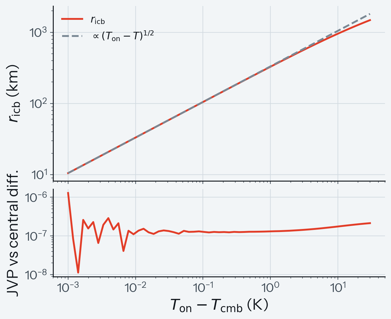
Figure 4. Inner-core growth below the onset. (a) Inner-core radius against undercooling, with the square-root law through the first point. (b) Relative difference between the implicit-function derivative and a central difference.
What the figure shows. In (a) the radius lies on the dashed square-root law at small undercooling and falls below it at the largest undercooling shown, the next order of the expansion. In (b) the difference between the two derivatives is largest at the smallest undercooling, next to the onset where the derivative diverges. A wrong derivative rule would show in (b) as a difference of order one. The latent and gravitational capacities use this derivative, so the cooling rate of a core with an inner core depends on it.
Pinned by tests/test_core_verification_page.py::test_inner_core_radius_grows_as_the_square_root_of_undercooling and tests/test_jax_dsdt_core_module.py::test_jacobian_core_column_matches_central_differences.
5. Nimmo (2015) Earth core budget
What is tested. The energy and entropy terms of the budget, the cooling rate and the inner-core growth rate, on a published parameter set for Earth's core.
Reference. Nimmo (2015, Table 2, p. 42) gives one parameter set for Earth's core:
| Input | Value |
|---|---|
| Central density | 12500 kg m\(^{-3}\) |
| Length scale \(L\) | 7272 km |
| CMB pressure | 139 GPa |
| Expansivity \(\alpha\) | \(1.25\times10^{-5}\) K\(^{-1}\) |
| Conductivity \(k\) | 130 W m\(^{-1}\) K\(^{-1}\) |
| Quadratic melting curve | \(T_{m0} = 2677\) K, \(T_{m1} = 2.95\times10^{-12}\) Pa\(^{-1}\), \(T_{m2} = 8.37\times10^{-25}\) Pa\(^{-2}\) |
| Latent heat | 750 kJ kg\(^{-1}\) |
| Light-element density jump | 560 kg m\(^{-3}\) |
Table 4 (p. 46) gives the present-day energy and entropy budget at \(T_c = 4180\) K for CMB heat flows of 15.2 and 12 TW without radiogenic heat. Table 5 (p. 46) gives the energy released since the onset, \(23\times10^{28}\) J (secular 11.6, latent 6.9, gravitational 4.4), and from it an inner-core age of 0.73 Gyr under a constant 10 TW.
Result. On aragog's Gaussian core with the third-order pressure, these inputs put the inner-core boundary at 1209 km and 328.5 GPa at 4180 K, against the 1220 km and 328 GPa of Table 2.
At 15.2 TW and 4180 K:
| quantity | Nimmo (2015) | aragog |
|---|---|---|
| \(Q_s\), \(Q_L\), \(Q_g\) (TW) | 6.1, 5.7, 3.4 | 6.06, 5.71, 3.43 |
| \(Q_k\) (TW) | 15.0 | 14.97 |
| \(E_s\), \(E_L\), \(E_g\), \(-E_k\) (MW K\(^{-1}\)) | 183, 327, 809, 450 | 182, 330, 820, 451 |
| \(-dT_c/dt\) (K Gyr\(^{-1}\)) | 104 | 103.3 |
| \(dr_\mathrm{icb}/dt\) (km Gyr\(^{-1}\)) | 1050 | 1075 |
Every energy and entropy term and the cooling rate agree to 1.3 percent at both heat flows (at 12 TW the cooling rate is 81.6 against 82 K Gyr\(^{-1}\)). The inner core grows 2.4 percent faster. The growth rate is \(|dr_\mathrm{icb}/dT_c|\) times the cooling rate: aragog's \(|dr_\mathrm{icb}/dT_c|\) is 10406 m K\(^{-1}\) against \(C_r = 10100\) m K\(^{-1}\) (Table 2), a factor of 1.030, and its cooling rate is 0.994 of Table 4. The CMB temperature has dropped by 59.3 K since the onset, against about 60 K (p. 43), and the melting temperature at the centre is 5808 K against 5800 K (Table 5).
Integrating aragog's capacities from 4180 K to the onset gives 22.2 (10.98, 6.83 and 4.42) \(\times10^{28}\) J and 0.70 Gyr. The secular term, the secular capacity times the drop, is 5 percent lower, and the chapter's own numbers account for most of the gap: its Table 4 secular capacity, \(Q_s\) over the cooling rate, times its 60 K drop gives 11.1 \(\times10^{28}\) J, 4 percent below its Table 5 value, while aragog's capacity is 1.0003 times that of Table 4 and its drop is 59.3 K.
The ages of Table 4, 0.59 and 0.75 Gyr, are not this integral: in our reading they are the drop since the onset times the present
over the heat flow, which on the numbers of Table 4 (\(4.6\times10^{27}\) J K\(^{-1}\)) and a 60 K drop gives 0.58 and 0.73 Gyr, within 3 percent of the table. The same quotient on aragog's state gives 0.574 and 0.727 Gyr, and the integral 0.464 and 0.587 Gyr, shorter because the latent and gravitational capacities rise from zero at the onset.
The bound is 2 percent on every energy and entropy term of Table 4 and on the cooling rate, at both heat flows.
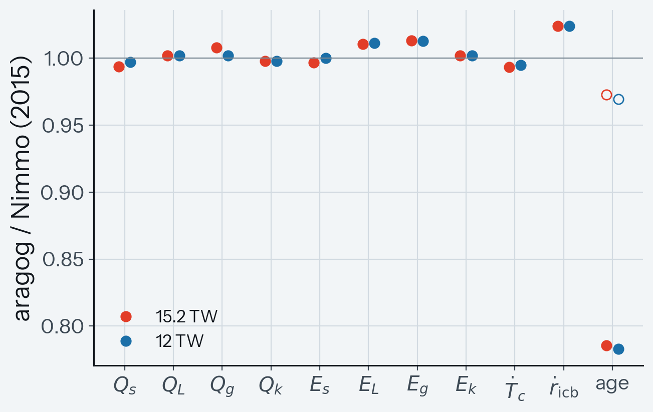
Figure 5. Ratio of aragog to Nimmo (2015, Table 4) at \(T_c = 4180\) K for 15.2 and 12 TW: the energy and entropy terms, the cooling and inner-core growth rates and the inner-core age. Filled circles give aragog's age as the integral of its capacity to the onset, open circles as the drop since the onset over the present cooling rate.
What the figure shows. The points of the eight energy and entropy terms and of the cooling rate lie close to the line at 1, at both heat flows; the growth rate lies above it. The filled circles of the age lie far below 1 and the open circles close to it: in our reading of the chapter, the gap comes from the definition of the age, not from the budget terms. A wrong term of the budget would move its point away from 1. These terms are computed from the capacities of the core_module budget, which set the core cooling and the inner-core growth of a run.
Limits. Four quantities are documented exceptions to the bound, each held at its measured value: the inner-core growth rate (1.024 of Table 4, from \(C_r\) and the cooling rate above), the inner-core age (0.786 and 0.783 of Table 4, which divides the drop by the present cooling rate), and \(W_s\) and \(W_\mathrm{tot}\) (0.947 and 0.967 of Table 5, from the chapter's own secular capacity above). Like the chapter, these numbers use the small-radius adiabat of section 1 (adiabat_mode = "small_radius"); the solver default integrates the exact gravity.
Pinned by tests/test_core_nimmo_benchmarks.py (the adiabat length scale, ICB state and adiabatic heat flow of the two models in Nimmo 2015, ch. 9.08, Table 2, their \(C_r\) from the caption of Figure 3, p. 211 (the value of model 2 is that of ch. 8.02, Table 2), and the ICB pressure and \(\tilde Q_T\) of ch. 8.02), tests/test_core_verification_page.py::test_the_earth_budget_meets_nimmo_tables_4_and_5 and ::test_page_numbers_match_the_values.
6. Budget terms against thermal_history
What is tested. The secular, latent and gravitational capacities and the conduction entropy sink, each against an independent core evolution code along one thermal history.
Reference. The leeds core model of thermal_history (Greenwood et al. 2021) computes the same budget with polynomial profiles, a trapezoid quadrature on a radial grid and its own inner-core growth. The comparison runs it on the Nimmo (2015, Table 2) core, with:
- the Gaussian density and adiabat given to it as the first 8 terms of their Taylor series in \(r^2\) (degree 14);
- the same quadratic melting curve without a light-element depression;
- a fixed latent heat of 750 kJ kg\(^{-1}\);
- complete rejection of the light element at the inner-core boundary;
- the CODATA gravitational constant aragog uses.
A core-only history starts at a CMB temperature of 4400 K under a fixed CMB heat flow of 10 TW; aragog's capacities are evaluated on each thermal_history state. Inputs, versions and licence are in tools/verification/data/.
Result. The secular term agrees to 1.4e-08 and the conduction entropy sink to 1.5e-07; the latent term agrees to 6.1e-04. The gravitational term differs by up to 3.8 %, because thermal_history enriches the outer core in the light element as the inner core grows (by the factor 1.039 at the end), while aragog holds the composition fixed; with that factor applied the two agree to 6.1e-04.
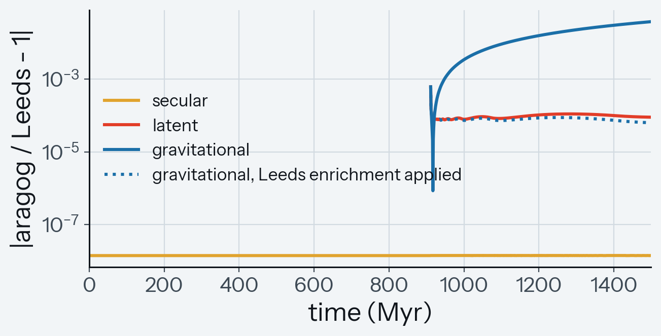
Figure 6. Relative difference of aragog's secular, latent and gravitational capacities from those of the leeds model of thermal_history along its 10 TW history on the same inputs; the dotted line applies thermal_history's outer-core enrichment to aragog's gravitational term.
What the figure shows. The secular difference is flat over the whole history, and the latent and gravitational differences start at the inner-core onset. The gravitational difference grows as the inner core grows, and the dotted line, with the enrichment applied, falls to the level of the latent line: the enrichment explains the gap. A wrong profile integral would put a term far above these levels from its first point. The cooling rate of a core_module core follows from the sum of these capacities.
Limits. aragog holds the composition of the outer core fixed, so its gravitational term differs from that of a model with enrichment by the amount above. The stratified layer is compared with thermal_history in section 13.
Pinned by tests/test_core_verification_page.py::test_budget_terms_match_the_thermal_history_table, and on the Nimmo (2015) state by tests/test_core_nimmo_benchmarks.py::test_budget_terms_match_thermal_history_cross_check and tests/test_core_entropy.py::test_entropy_capacities_match_thermal_history.
7. Dynamo criterion and field strength
What is tested. The entropy budget gives the entropy production available to the dynamo,
positive when the core can sustain a dynamo. The field strength follows the energy-flux scaling of Christensen et al. (2009, eq. 2),
with \(c = 0.63\) and the efficiency factor
the first for a constant total heat flow \(4\pi r^2 q_c\), the second for a convected flux that vanishes at the outer boundary (p. 168). With \(f_\mathrm{ohm} = 1\), the upper end of \(f_\mathrm{ohm} \le 1\) (p. 167), the field is the largest the scaling allows for that flux.
Reference. The references are the two efficiency factors that Christensen et al. print for their Earth inputs (\(\alpha = 1.35\times10^{-5}\) K\(^{-1}\), \(g = 10.7\) m s\(^{-2}\), \(R = 3480\) km, \(c_p = 840\) J kg\(^{-1}\) K\(^{-1}\)), Nimmo's (2015, p. 46) minimum heat flow for a present-day dynamo without radiogenic heat, and the internal field of Earth from Christensen et al.'s dipole field of 0.26 mT at the dynamo surface and their ratio of about 7 between the total and the dipole field (p. 168).
Result. With Christensen et al.'s Earth inputs the two factors are 0.527 and 0.269, against the printed 0.52 and 0.27; on the Nimmo (2015) core the constant-flux factor is 0.484, lower mainly through the lower expansivity (\(1.25\times10^{-5}\) K\(^{-1}\); the CMB gravity, 10.6 m s\(^{-2}\), accounts for under 1 percent). On that core at \(T_\mathrm{cmb} = 4180\) K the adiabatic heat flow is 14.97 TW and the entropy margin vanishes at 5.14 TW, against Nimmo's minimum of about 5 TW. Between these two heat flows the margin is positive but no flux is superadiabatic, so the field estimate is zero although the entropy budget allows a dynamo. At 17 TW the core field is 1.10 mT, the order of magnitude of the 1.82 mT for Earth.
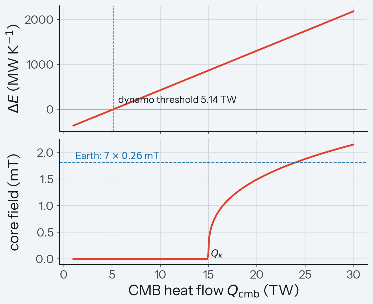
Figure 7. Dynamo criterion and field strength on the Nimmo (2015) core at \(T_\mathrm{cmb} = 4180\) K. (a) Entropy margin against CMB heat flow, with the threshold where it vanishes. (b) Volume-averaged core field from Christensen et al. (2009, eq. 2), with Earth's estimated internal field. The field is zero up to the adiabatic heat flow \(Q_k\), 15.0 TW, so also from 5.1 TW, where the margin turns positive, to \(Q_k\).
What the figure shows. In (a) the margin rises with the CMB heat flow and crosses zero at the threshold. In (b) the field is zero up to \(Q_k\) and rises steeply above it, and crosses the dashed line of Earth's estimate inside the plotted range. A wrong sign of the conduction sink \(E_k\) would move the zero crossing in (a), and a field computed from the total heat flow would be nonzero below \(Q_k\) in (b). The entropy margin and the field strength that PROTEUS writes for a core_module run come from the two relations of this section.
Limits. Christensen et al. derive the efficiency factors for Earth's core with an inner core of 0.35 of the core radius, \(L = D\), constant density and thermodynamic properties and gravity linear in radius (pp. 167 and 168); aragog applies them at every inner-core size. Their \(q_o\) is the effective convected flux at the inner boundary, compositional driving included, scaled to the outer radius (p. 167); aragog takes the superadiabatic part of the CMB heat flow over the CMB area, a thermal flux only, so here \(q_o\) departs from their definition. With \(q_o\) defined differently, the field comparison is an order-of-magnitude check only.
Without the resolved shell (stratification = false) the efficiency factors of \(\Delta E\) use \(T_\mathrm{cmb}\), the convecting adiabat extended to the CMB. Under a stratified layer the reference of the whole-core entropy balance is the actual CMB temperature (Greenwood et al. 2021, eq. 4 and p. 9), which aragog does not resolve without the shell and which lies between \(T_\mathrm{cmb}\) and \(T_a(r_s)\) at the base of the layer; \(\Delta E\) is then the upper end of that bracket. With the resolved shell the reference is the temperature of the top shell cell (core_bc.md).
Pinned by tests/test_core_entropy.py::test_chr09_efficiency_factors_reproduce_printed_values, ::test_field_scaling_bounds_and_earth_magnitude and ::test_dynamo_threshold_and_margin.
8. Iron melting curve
What is tested. The pure-iron melting curve is the two-branch Simon-Glatzel fit of Anzellini et al. (2013, eqs. 2 and 3, p. 466); this is the PALEOS prescription. On the \(\gamma\)-Fe branch, with \(T_0 = 1991\) K and \(P_0 = 5.2\) GPa,
and on the \(\epsilon\)-Fe branch, from the \(\gamma\)-\(\epsilon\)-liquid triple point at 98.5 GPa and 3712 K,
with \(P\) in GPa, \(T_m\) the melting temperature and \(P_\mathrm{TP}\) and \(T_\mathrm{TP}\) the pressure and temperature of the triple point. The two branches meet with a jump at the triple point, which a \(C^2\) smootherstep over a 3 GPa half-width removes. Light elements depress the curve by the factor \(1 - \mathrm{depression} \times x\).
Reference. The reference is the unblended fit: the two branches as printed, and the PALEOS source for the pure-iron values.
Result. The jump of the two branches at the triple point is 0.725 K; the blended curve departs from the branches by at most 0.361 K and equals them exactly outside the blend. The depression factor is 0.88 for \(x = 0.1\) and a depression of 1.2. The pure-iron curve gives 4192.0 K at 136 GPa and 6229.2 K at 330 GPa.
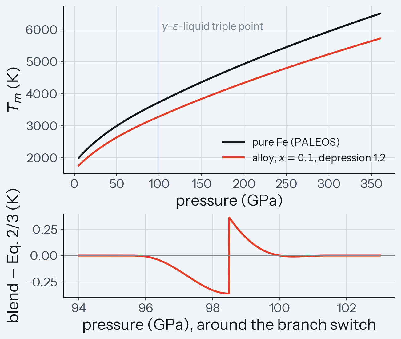
Figure 8. Iron melting curve. (a) Pure-iron and alloy melting temperature against pressure, with the triple point marked. (b) Blended curve minus the unblended Anzellini et al. (2013) branches around the triple point; the jump is that of the unblended fit.
What the figure shows. In (a) both curves rise smoothly through the triple point, and the alloy curve lies below the pure-iron curve at every pressure. In (b) the difference from the unblended branches is zero outside the blend and largest on both sides of the triple point; its jump there is the jump of the unblended fit, so the blended curve is continuous. Without the blend, the melting temperature would jump at the triple point, and so would the inner-core radius of a core whose inner-core boundary passes that pressure. The onset temperature and the inner-core radius of a core_module run with the iron curve follow from it.
Limits. The depression is a model choice, not part of the Anzellini fit.
Pinned by tests/test_core_melting.py::test_pure_iron_pins_against_the_paleos_source, ::test_branch_switch_matches_unblended_outside_transition and ::test_branch_switch_deviation_and_c1_continuity.
9. A CVODE solve across the inner-core onset
What is tested. The coupled right-hand side carries the core temperature as a state, so CVODE integrates the core through the onset, where the latent capacity rises as a square root. The check compares the core heat change that the solver books with the CMB heat that it books.
Reference. The quadratic melting curve of section 5 at 1.5 times its \(T_{m0}\) (4015.5 K) puts the onset above the mantle base. The call starts with a core 2 K above the onset over a partly molten mantle base and lasts 4 yr. The bound is \(10^{-6}\) for a core without a layer solved alone.
Result. The core cools from 6414.4 K to 6409.5 K, through the onset at 6412.4 K, and grows an inner core of 244 km. At a solver rtol of \(10^{-10}\) (atol stays at its floor of \(10^{-8}\)) the solver books the core heat change as the heat-content difference, and that change matches the CMB heat it books to 5.7e-07, within the bound. The CMB heat reconstructed from the 71 output times by the trapezoid rule matches to 5.6e-04, the error of that sampling.
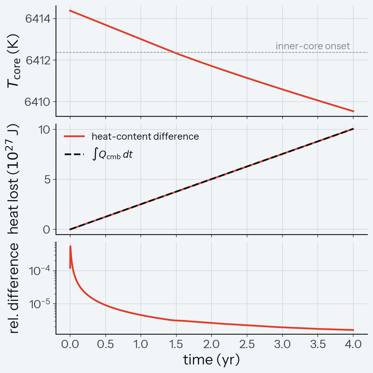
Figure 9. A CVODE solve through the inner-core onset. (a) Core temperature against time, with the onset temperature. (b) Core heat lost from the heat-content difference and from the time integral of the CMB heat flow. (c) Relative difference between the two curves in (b).
What the figure shows. In (a) the core temperature crosses the onset temperature during the call. In (b) the two curves of the heat lost lie on each other, and (c) gives their difference, which is the sampling error of the trapezoid rule over the output times and is largest at the first outputs. A core temperature that did not follow the CMB heat flow through the onset would separate the curves in (b). The core energy ledger of a core_module run rests on this closure.
Limits. At the default rtol of \(10^{-8}\) the CMB heat matches to 1.5e-06, so a call across the onset needs the tighter tolerance to meet that bound. Panel (c) does not show the closure of the booked ledger, only the sampled reconstruction.
Pinned by tests/test_entropy_solver_core_module_smoke.py::test_core_module_cvode_solve_crosses_the_inner_core_onset and tests/test_core_verification_page.py::test_a_cvode_solve_across_the_onset_closes_its_heat.
10. A core thermal history against thermal_history
What is tested. The core-only history of section 6 tests the integrated evolution rather than the terms.
Reference. aragog integrates its cooling rate under the same fixed 10 TW CMB heat flow with LSODA (SciPy solve_ivp) at a relative tolerance of \(10^{-10}\) and an absolute tolerance of \(10^{-8}\) K, and thermal_history steps it with its own fixed 1 Myr steps.
Result. Over 1499 Myr the CMB temperatures differ by at most 0.119 K. The centre temperatures, on the same adiabat, differ by at most 0.163 K, the CMB difference times the adiabat ratio, and the final inner-core radii by 0.13 %, within the bounds of 0.2 K for the CMB temperature, 1 K for the centre temperature and 1 % for the radius.
| Quantity | aragog | thermal_history |
|---|---|---|
| Inner-core nucleation (Myr) | 911 | 911, on its 1 Myr grid |
| Final inner-core radius (km) | 1122.8 | 1121.4 |
The inner-core age is 588 Myr in both.
Before the onset the CMB temperatures agree to 2.2e-06 K. The difference appears at the onset, 6.5e-04 K at the first step, rises to 0.024 K, changes sign at 1196 Myr and reaches its largest magnitude at the end, at 1499 Myr (aragog minus thermal_history throughout).
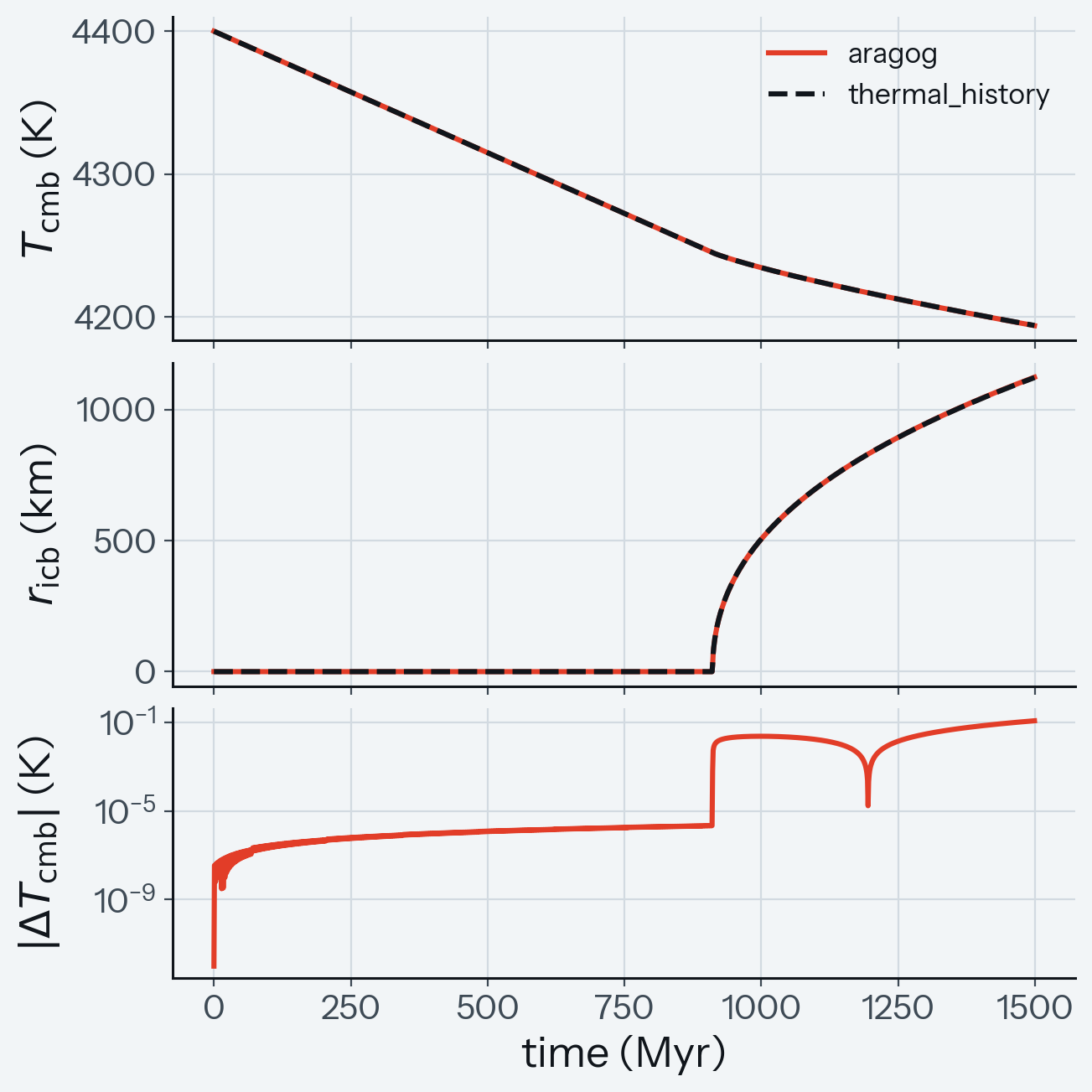
Figure 10. Core-only thermal history under a fixed 10 TW CMB heat flow. (a) CMB temperature from aragog and thermal_history. (b) Inner-core radius. (c) Absolute difference of the CMB temperatures.
What the figure shows. In (a) and (b) the two models lie on each other; the cooling slows where the inner core starts to grow. In (c) the difference is small before the onset, jumps at the onset, passes through zero at the sign change and is largest at the end. A wrong secular capacity would give a difference that grows from the start of the history, not from the onset. The CMB temperature and the inner-core radius are the outputs of the core model that a core_module run reports.
Limits. We attribute the jump at the onset to thermal_history's explicit step, which crosses the start of the latent release in one step, and the later drift to the outer-core enrichment of section 6, which shifts the gravitational term; neither cause is tested separately.
Pinned by tests/test_core_verification_page.py::test_core_history_matches_the_thermal_history_table.
11. Coupled PROTEUS case
What is tested. Coupled PROTEUS runs test the sign of the CMB flux against the core-mantle temperature contrast, the closure of the core ledger against the CMB heat, and the dependence of the CMB flux on the mantle mesh.
Reference. A coupled PROTEUS run of a 1 Earth-mass planet that starts fully molten runs to mantle solidification twice, once with core_bc = "core_module" and once with energy_balance, whose CMB flux follows the mantle-side entropy gradient. The configuration is tools/verification/data/coupled_config.toml:
- Zalmoxis structure;
- the CVODE solver;
- the PALEOS iron curve with a light-element depression;
- no stratification;
- the PALEOS-2phase MgSiO\(_3\) mantle tables.
The same configuration at 3 and 5 Earth masses (planet.mass_tot) and at 1 Earth mass with interior_energetics.rtol = 1e-10 gives the core ledgers in tools/verification/data/coupled_ledger_*.csv.
The coupled tables of the plotted columns are in tools/verification/data/, each with the PROTEUS and aragog commits of its run in its header. The core_module tables come from an inversion of the layer's temperature that agrees with the one described in the core boundary condition to rounding, except for a layer mean temperature within about \(3 \times 10^{-11}\) K of a phase-boundary temperature, where the EOS tables hold the temperature flat.
Flux sign
With core_module no row of the 1 Earth-mass run has a CMB flux against the core-mantle temperature contrast. The same holds for the 3 and 5 Earth-mass runs and for a 1 Earth-mass run with the Wolf and Bower (2018) mantle. The table gives the rows of each run, the rows with a flux against the contrast (wrong sign), the largest contrast, the rows with zero flux and the contrast of those rows:
| Run | Rows | Wrong sign | Largest contrast (K) | Zero flux | Contrast at zero flux (K) |
|---|---|---|---|---|---|
| 1 \(M_\oplus\) | 661 | 0 | 823 | 1 | 4.8e-08 |
| 3 \(M_\oplus\) | 795 | 0 | 1928 | 1 | 0 |
| 5 \(M_\oplus\) | 695 | 0 | 2428 | 1 | 1.0e-06 |
| 1 \(M_\oplus\), Wolf and Bower (2018) mantle | 217 | 0 | 712 | 1 | 0 |
coupled_flux_<case>.csv holds the rows of the last three runs.
With energy_balance the core runs 7.7 to 10.0 K colder than the mantle side of the CMB, and the flux carries heat out of it on all 681 rows.
With the boundary layer's properties at its mean temperature, the core_module core follows the mantle: it cools to 5251 K while the mantle side of the CMB cools to 4428 K, which gives the largest contrast of its row in the table, and the CMB flux is still 8.0 W m\(^{-2}\) at 500 kyr. The mantle reaches a melt fraction of 0.05 at 661 kyr with core_module and at 665 kyr with energy_balance, which feeds core heat into the mantle throughout.
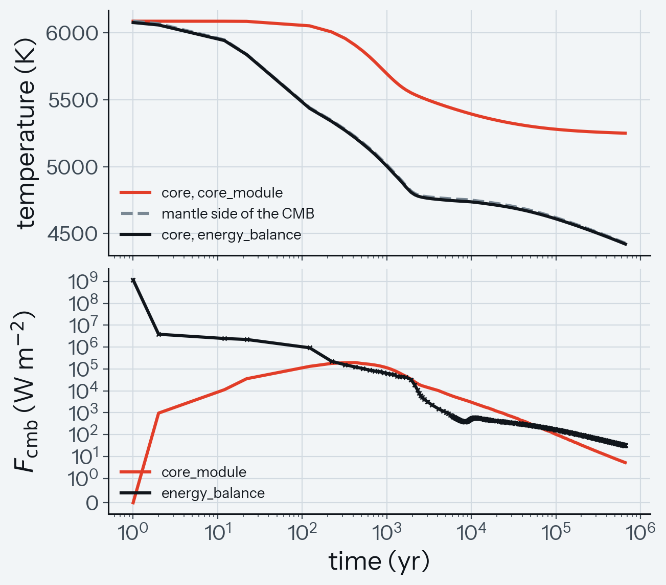
Figure 11. A coupled PROTEUS run to mantle solidification with the core_module and the energy_balance core boundary conditions. (a) Core temperature in both runs and the mantle side of the CMB, which cools alike in both. (b) CMB heat flux; crosses mark rows where the flux carries heat against the core-mantle temperature contrast.
What the figure shows. In (a) the energy_balance core lies on the mantle side of the CMB, while the core_module core stays hotter and cools more slowly. In (b) every row of the energy_balance line has a cross and no row of the core_module line has one; the core_module flux starts at zero, where the core starts at the mantle temperature. A flux law with a wrong sign would put crosses on the core_module line. The sign of the CMB flux decides whether the core heats or cools the mantle base of a run.
Core ledger closure
The table gives the cumulative residual of the core ledger relative to the cumulative CMB heat, the share of the summed absolute call residuals that comes from the call from 22 to 122 yr, and the bound for each run. The bound applies to the cumulative residual after the first kyr and at the end.
| Run | residual at the end | largest after 1 kyr | share of the call from 22 to 122 yr | bound |
|---|---|---|---|---|
| 1 \(M_\oplus\), rtol \(10^{-8}\) | 1.5e-07 | 1.9e-07 | 0.04 | \(10^{-6}\) |
| 1 \(M_\oplus\), rtol \(10^{-10}\) | 4.7e-08 | 6.1e-08 | 0.08 | \(10^{-6}\) |
| 3 \(M_\oplus\), rtol \(10^{-8}\) | 1.8e-07 | 2.4e-07 | 0.06 | \(5 \times 10^{-6}\) |
| 5 \(M_\oplus\), rtol \(10^{-8}\) | 1.5e-07 | 2.0e-07 | 0.09 | \(5 \times 10^{-6}\) |
The call from 22 to 122 yr gives 4 to 9 percent of the summed call residuals. The bound is \(5 \times 10^{-6}\) for the last two runs of the table and \(10^{-6}\) for the 1 Earth-mass runs and for a core without a layer solved alone (section 9).
The first call of nonzero length, from 1 to 2 yr, closes to 1.5e-04 of its own CMB heat at 1 Earth mass and to 1.0e-04 to 1.1e-04 in the other runs; the source of this error is not established, and the test holds it below \(3 \times 10^{-4}\). tests/test_entropy_solver_core_module_smoke.py::test_chained_cvode_calls_close_the_core_ledger makes calls ending at the same times on a core solved alone and closes each to \(10^{-6}\); it does not reproduce this error, and the bounds of the table are checked on the stored runs, not on the current solver.
Cores without an inner core and the top-down case
None of the 1, 3 and 5 Earth-mass runs grows an inner core. The cores are coldest at the end of each run, above their inner-core onsets (the budget rebuilt from the core profile of each run in coupled_core_structure.csv), so these runs test the secular capacity only:
| Run | Core temperature at the end (K) | Inner-core onset (K) |
|---|---|---|
| 1 \(M_\oplus\) | 5251 | 4028 |
| 3 \(M_\oplus\) | 6902 | 4598 |
| 5 \(M_\oplus\) | 8187 | 4266 |
Section 9 takes a CVODE solve through the onset, and tests/test_entropy_solver_core_module_smoke.py::test_a_cvode_call_through_onset_and_freeze_out_closes_its_heat takes one through the onset and freeze-out, with an entropy of fusion of 0.17 J kg\(^{-1}\) K\(^{-1}\) and no gravitational term, so that one call crosses the whole band.
With the Earth values of the thermal expansivity and the heat capacity in the core adiabat (below), at 3 and 5 Earth masses the melting curve reaches the adiabat at the CMB, at 5217 K and 6865 K, before it reaches it at the centre, so these cores would freeze from the top down; the order of the two temperatures depends on that adiabat. The budget books latent and gravitational heat only for an inner core that grows from the centre, so a call that enters a top-down or snow regime raises an error; the energetics of those regimes are not modelled. ::test_a_core_that_freezes_from_the_top_is_refused takes a solver call into the top-down regime, and tests/test_core_nimmo_benchmarks.py::test_model1_printed_parameters_break_bottom_up_topology gives a snow state to the guard that the solver calls. The runs end above these temperatures.
Pressures and extrapolation
| Run | CMB pressure (GPa) | Centre pressure (GPa) |
|---|---|---|
| 1 \(M_\oplus\) | 103 | 341 |
| 3 \(M_\oplus\) | 298 | 1045 |
| 5 \(M_\oplus\) | 516 | 1837 |
The structure EOS of the core is the PALEOS iron table, which spans pressures up to 100 TPa and so covers these. The melting curve is the fit of section 8, to melting points that Anzellini et al. (2013) measured from 50 to 200 GPa: it is an extrapolation at the centre of every run and at the CMB of the 3 and 5 Earth-mass runs, and so are the onset and freeze-out temperatures that follow from it there. The budget uses the Earth values of the thermal expansivity, \(1.35 \times 10^{-5}\) K\(^{-1}\), and the heat capacity, 840 J kg\(^{-1}\) K\(^{-1}\), at every mass.
Mesh dependence of the CMB flux
The 1 Earth-mass core_module run at 40, 80, 160 and 320 mantle levels (interior_energetics.num_levels), and at 80 levels with interior_energetics.rtol = 1e-10, tests how the CMB flux depends on the mantle mesh through basal freezing, the time \(t_\mathrm{bf}\) at which the melt fraction of the lowest mantle node falls through 0.5 (coupled_mesh_convergence.csv). At 320 levels basal freezing comes at 1327 yr, with a CMB flux of 7.48e+04 W m\(^{-2}\).
From 160 to 320 levels the changes are within the bounds of 5 % for the times and fluxes and 10 K for the temperatures:
| Quantity | Change from 160 to 320 levels |
|---|---|
| \(t_\mathrm{bf}\) | 0.62 % |
| Core temperature at \(t_\mathrm{bf}\) | 1.34 K |
| Core temperature at the end | 0.11 K |
| CMB flux at 10 yr | 0.029 % |
| CMB flux at 100 yr | 0.0044 % |
| CMB flux at 1000 yr | 0.041 % |
| CMB flux at \(t_\mathrm{bf}\) | 0.80 % |
After basal freezing the flux converges too: at twice and four times \(t_\mathrm{bf}\) and at 10, 100 and 500 kyr it changes by at most 1.1 % from 160 to 320 levels, by at most 4.0 % from 80 to 160 and by at most 7.8 % from 40 to 80; a flux set by conduction across the half cell would double with each doubling. At 500 kyr it is 8.27, 7.99, 8.16 and 8.12 W m\(^{-2}\) at 40, 80, 160 and 320 levels, and the core cools by 370 to 376 K from \(t_\mathrm{bf}\) to the end.
The tighter tolerance at 80 levels changes the bounded fluxes and times by at most 3.1e-05 and the temperature at \(t_\mathrm{bf}\) by 0.0054 K. The flux of a row is the mean over the call that ends at it, and the fluxes at a given time are linear between the row times; at 100 kyr the calls of the two runs last 1.1 and 0.16 kyr, so their fluxes there differ by 0.4 %, against 5.0e-05 with each call mean placed at the middle of its call (from the CMB heat of each call in coupled_ledger_1me*.csv).
Limits and tests of the coupled case
Limits. The liquid heat capacity of the PALEOS-2phase mantle tables is too large (PALEOS issue 6), so these runs test the core ledger and the flux sign, not the mantle's cooling history. The limits of each part are stated with it: the first-call error of the ledger, the secular capacity as the only capacity tested, the top-down case, and the extrapolation of the melting curve.
Pinned by tests/test_core_verification_page.py::test_coupled_tables_reproduce_the_page, which recomputes these numbers from the tables and holds them to the bounds above; the runs themselves need PROTEUS and are not repeated by the test suite.
12. NumPy and JAX right-hand sides and the analytic Jacobian
What is tested. The solver evaluates the coupled right-hand side in NumPy and, for CVODE's analytic Jacobian, in JAX; the two must agree, and the JAX Jacobian must equal the derivative of that right-hand side. The two evaluate the same equations except for the single-phase thermal expansivity: NumPy reads it from the thermal_exp tables, JAX derives it from the identity
Reference. Each right-hand side is the reference of the other, and a central difference of \(\dot T_\mathrm{core}\) is the reference of the analytic Jacobian entry \(\partial \dot T_\mathrm{core}/\partial T_\mathrm{core}\). The comparison runs on a 10-node mesh with the core in three states (inside the growth band, 100 K above the onset, and stratified with the core 50 K above the mantle), with the NumPy expansivity from the identity as well. These states put the mantle cells in the mush, where the composite expansivity applies and the tables do not enter; a fourth comparison puts the mantle above its liquidus at every node.
Result.
| Comparison | Relative difference |
|---|---|
| Right-hand sides, largest over the components, first two states | 1.4e-12 |
| Right-hand sides, largest over the components, with the layer, whose core rate is ill-conditioned (section 13) | 2.0e-10 |
| Right-hand sides over a liquid mantle, largest over the components, with the identity | 2.8e-14 |
| Right-hand sides over a liquid mantle, largest over the components, with the tables | 1.7e-04 |
| Jacobian entry against a central difference at the best step, in the growth band | 1.6e-11 |
| Jacobian entry against a central difference at the best step, with the layer | 1.5e-11 |
The difference with the tables is the difference of the two single-phase expansivities on these tables, which NumPy reads from the tables for the mantle cells and for the boundary layer when they are present; on the two 1350 by 280 sets the same comparison, run separately from the script, gives \(6.1 \times 10^{-5}\) and \(2.1 \times 10^{-5}\). The best step is the one that balances truncation and rounding; above the onset the core is colder than the mantle base, the flux is on its linear conduction branch, and the difference stays at rounding for every step.
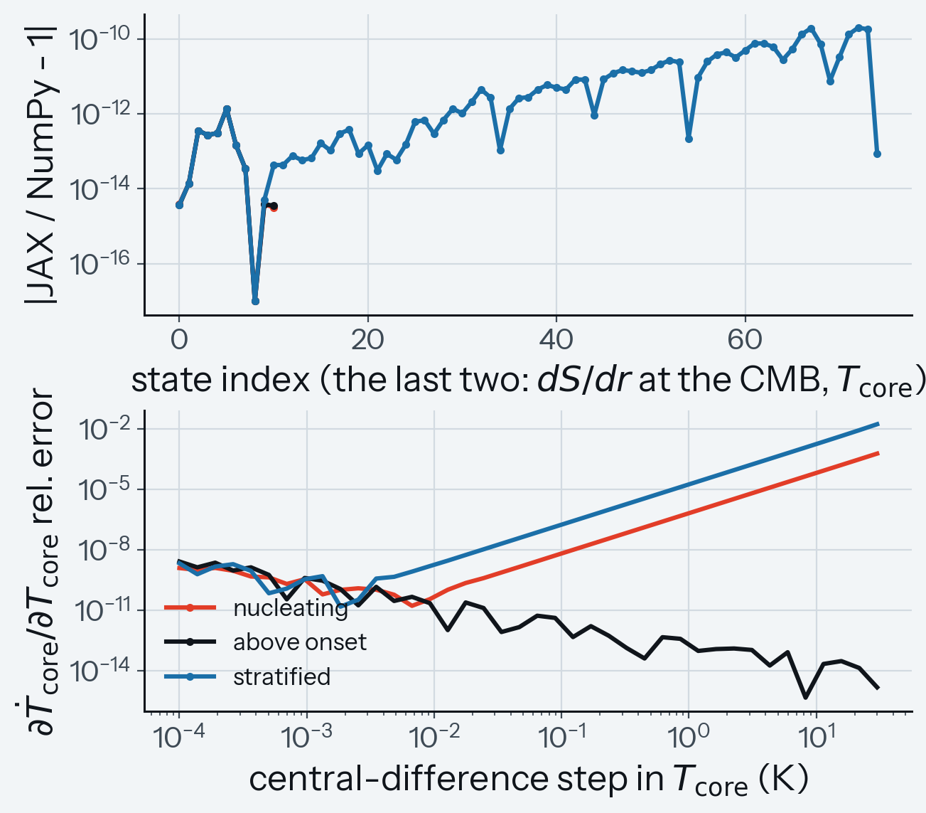
Figure 12. Agreement of the NumPy and JAX core right-hand sides. (a) Relative difference per state component, the entropy cells first and the CMB entropy gradient and core temperature last, in three core states. (b) Relative error of a central difference of \(\dot T_\mathrm{core}\) against the analytic Jacobian entry, against the difference step.
What the figure shows. In (a) the stratified state has the most components, its shell cells, and the largest differences, at the level of the table above; the lines of the two other states end after the entropy cells and the two boundary slots. In (b) the error of the central difference falls with the step to a minimum and rises again at small steps, where rounding takes over; above the onset it stays at rounding. A wrong Jacobian entry would give an error that does not fall with the step. With use_jax_jacobian set, as in PROTEUS, CVODE builds the implicit steps of a core_module run on this Jacobian.
Limits. In the three core states the CMB flux is the conduction across the half cell, and in runs separate from the script the numbers of this section do not change when the expansivity of the boundary layer is multiplied by 1.5 in both NumPy and JAX; tests/test_jax_dsdt_core_module.py::test_jacobian_core_column_matches_central_differences checks the boundary-layer flux instead, with the Jacobian columns of the core temperature and the bottom cell against central differences for a core 300 K above a base at melt fraction 0.66, where the test asserts a flux above \(10^4\) W m\(^{-2}\).
Pinned by tests/test_jax_dsdt_core_module.py::test_boundary_slots_match_numpy_on_a_five_node_mesh, ::test_jacobian_core_column_matches_central_differences and ::test_jacobian_carries_boundary_couplings.
13. Stable layer against thermal_history
What is tested. The resolved layer of stratification = true is compared with the leeds_thermal model of thermal_history (Greenwood et al. 2021) on the core of section 6, which starts on the adiabat at a CMB temperature of 4400 K. The conducted adiabatic flow at the CMB is 15.8 TW. Under a CMB flow below it, the top of the core takes up more heat by conduction along the adiabat than the CMB removes, and a warm stable layer forms; the CMB removes 8 or 12 TW, adds 2 TW, or removes nothing. Under a flow above it, an existing layer erodes.
Reference. aragog resolves the outer core above 0.4 \(r_\text{cmb}\) in 64 cells with the default mixing constants; mixing acts only where the temperature falls outward faster than the adiabat, so a subadiabatic region conducts only. leeds_thermal instead moves the base of its layer by a stability check after each step. The layer depth is defined the same way on both sides: the depth below the CMB where the excess over the convecting adiabat falls to 0.1 of its value at the top, which for aragog is the centre of its top cell. The CMB temperature of aragog that is compared with leeds_thermal is the temperature of that cell (core_T_top), not the state \(T_\text{cmb}\) of the convecting adiabat. aragog integrates the convecting core and the shell alone with SciPy BDF at a relative tolerance of 1e-11.
In the four cases with a fixed flow, until the inner core of leeds_thermal forms at 588 Myr, its centre temperature differs by at most 0.33 K between the flows and its layer depth from 200 Myr on by at most 1.4 %; the CMB temperature depends on the flow throughout.
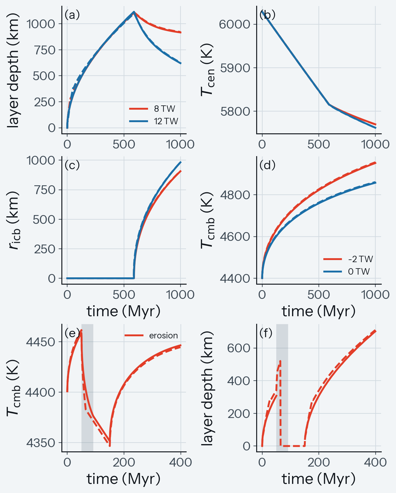
Figure 13. The resolved stable layer of aragog (solid) against the leeds_thermal model of thermal_history (dashed). (a) Layer depth at 0.1 of the top excess over the adiabat, (b) centre temperature and (c) inner-core radius under a CMB flow of 8 and 12 TW to 999 Myr; (d) CMB temperature under -2 and 0 TW. (e) CMB temperature and (f) layer depth in the erosion case to 399 Myr; the shaded window runs from the rise of the flow at 50 Myr to the time aragog's shell mixes completely, and aragog's depth is not drawn while the mixing acts below its top cell, where the depth at 0.1 of the top excess has no meaning.
What the figure shows. In (a) to (d) the solid and dashed lines lie close to each other: the layer grows until the inner core forms and thins after it, and the CMB warms under the two flows of (d). In (e) and (f) the models differ inside the shaded window, where each removes the layer in its own way, and form a new layer of similar depth after the flow falls back. A shell that lost or gained heat would separate the centre temperatures in (b). The layer base (core_layer_base) and the top temperature (core_T_top) that a stratified core_module run reports come from this shell.
Fixed flows
| CMB flow | max \(\lvert\Delta T_\text{cmb}\rvert\) (K) | max \(\lvert\Delta T_\text{cen}\rvert\) (K) | depth ratio | onset aragog (thermal_history) (Myr) | \(r_\text{icb}\) at 999 Myr |
|---|---|---|---|---|---|
| 8 TW | 2.88 | 0.62 | 0.79 to 1.13 | 590 (588) | 0.20 % |
| 12 TW | 2.23 | 0.62 | 0.82 to 1.39 | 589 (588) | 0.05 % |
| -2 TW | 4.11 | 1.24 | 0.79 to 1.01 | 592 (589) | 0.24 % |
| 0 TW | 3.88 | 0.93 | 0.79 to 1.01 | 591 (589) | 0.15 % |
For the four fixed flows the bounds are:
- 5 K on the CMB temperature;
- 10 K on the centre temperature;
- a factor of 1.5 on the layer depth where both layers are thicker than 10 km after the first Myr;
- 2 % on the inner-core radius at the last sample (999 Myr);
- 5 % on its onset time.
The extremes of the depth ratio fall in the first 51 Myr, while the layer is thin; from 300 Myr on the two depths agree to within 1.5 % (Figure 13a). The CMB temperature difference reaches its largest value between 36 and 69 Myr, with aragog colder. aragog reports its top cell as the CMB temperature; the centre of that cell lies 1000 m below the CMB, where the adiabat of the starting core is 0.80 K above the CMB temperature, so aragog starts that much warmer.
Tolerance and reproducibility
Where BDF stalls, the integration restarts from its last accepted state; the shell runs of this section, at every tolerance and mixing constant, restart 1 time in all, a count that can differ between platforms. Between runs at 1e-11 and 1e-12 the centre temperature differs by at most 0.27 K.
In runs separate from the script, whose values, commits and platforms are in tools/verification/data/stable_layer_spread.json, that difference comes from the -2 TW case: a start temperature changed in its last bit lowers its largest centre-temperature difference from thermal_history from 1.24 K to 0.99 K, the tolerance of 1e-12 to 0.99 K, and the two changed runs agree to 0.008 K. In the other cases the last-bit change moves that difference by 0.024 K or less, the inner-core radii by 2.8e-05 of themselves or less (8.3e-05 at -2 TW) and the largest late depth difference by 0.075 percentage points. On Linux the 8 TW difference of the table above is 0.69 K, 0.07 K above the value here. The centre-temperature differences therefore reproduce only to within changes of up to 0.25 K, and the page test holds them to 0.6 K at -2 TW and to 0.2 K in the other cases.
At a relative tolerance of 1e-8 the comparison has not converged: the centre temperature then differs from thermal_history by up to 8.7 K and the inner-core onset by up to 26 Myr.
The heat rates of the core and the shell sum to the CMB flow at every sample to 5.0e-16 of the conducted adiabatic flow or better, in every case; this is a property of the discretisation (the shell fluxes telescope and the core uses one effective capacity), not of the integration.
Coupled to the mantle solver, a 5 yr CVODE call that heats a stratified core from above closes its heat against the CMB heat, in runs separate from the script, to \(1.9 \times 10^{-6}\) or \(8.2 \times 10^{-6}\), a choice a rounding-level change of the input makes (\(7.7 \times 10^{-6}\) or \(8.2 \times 10^{-6}\) with the exact adiabat and the boundary-layer properties at the mean temperature), because the stratified core rate moves by \(1.5 \times 10^{-6}\) of itself under a \(10^{-14}\) change of the shell temperatures; tests/test_entropy_solver_core_module_smoke.py::test_a_core_heated_from_above_warms_its_top_and_closes_its_heat holds that call to \(10^{-5}\).
Erosion case
In the erosion case the CMB flow is 8 TW to 50 Myr, 25 TW to 150 Myr and 8 TW again to 400 Myr. The two models remove the layer in different ways.
In aragog the face below the top cell mixes within the first Myr of the higher flow (at 51 Myr), and a mixed region then grows down from the CMB over the remaining stable part until the whole shell mixes at 92 Myr; the heat stored in the shell at 50 Myr, 1.22e+28 J, drains through the excess of the CMB flow over the conducted adiabatic flow, 9.31 TW on average, in 41.7 Myr against the 42 Myr from 50 to 92 Myr.
In leeds_thermal the layer at the CMB conducts until its excess over the adiabat at the top reaches zero at 65 Myr, where its depth at 0.1 of that excess vanishes; its stability check removes the layer base at 66 Myr.
The CMB temperature during erosion is a model difference, without a bound: from the rise of the flow aragog's mixed top stays warmer than the conducting top of leeds_thermal, by up to 19.6 K at 65 Myr, when the top excess of leeds_thermal reaches zero, and from 92 Myr until the flow falls at 150 Myr the two CMB temperatures stay 4.75 K apart (varying by 0.003 K), an offset that forms during erosion.
Once its shell has mixed completely, aragog's centre temperature stays within 0.003 K of that of aragog without a layer under the same flows until the flow falls, against 9.06 K below it at the rise of the flow, so the heat stored in the shell returns to the convecting core. The centre temperatures of aragog and leeds_thermal differ by up to 5.43 K. After the flow falls back to 8 TW a new layer forms in both models, 702 km deep in aragog and 710 km in leeds_thermal at 399 Myr (Figure 13e, f).
Mixing constants
The two mixing constants are a model uncertainty, not a fitted quantity. Changing layer_k_mix or layer_g_mix by a factor of 10 either way changes the centre temperature of the 8 and 12 TW cases by at most 0.17 K, which the last-bit change of the start temperature moves by 0.13 K, so the comparison does not resolve this sensitivity and these changes are not reproduced (the page test checks only that each setting changes the centre temperature, by less than 1 K), and their layer depth by at most 0.3 %, which the tolerance of 1e-12 lowers to 0.12 %; the time at which the eroding shell mixes completely moves by 0 Myr at the sampling of the reference table.
Limits and tests of the stable layer
Limits. This comparison runs on SciPy BDF; in the solver, an eroding layer stalls CVODE at its default tolerances (see the core boundary condition). The limits of each part are stated with it: the reproducibility of the centre temperatures, the unconverged comparison at the looser tolerance, the CMB temperature during erosion, and the unresolved sensitivity to the mixing constants.
Pinned by tests/test_core_verification_page.py::test_the_stable_layer_meets_the_thermal_history_bounds; the analytic limits of the shell by tests/test_core_layer.py::test_a_young_layer_follows_the_erfc_solution_of_a_half_space, ::test_a_steady_layer_reaches_the_quasi_static_depth and ::test_mixing_keeps_a_superadiabatic_shell_on_the_adiabat; a resumed solve by tests/test_entropy_solver_core_module_smoke.py::test_a_resume_restarts_the_shell_where_the_previous_solve_ended.
References
- Anzellini, S., Dewaele, A., Mezouar, M., Loubeyre, P., & Morard, G. (2013). Melting of iron at Earth's inner core boundary based on fast X-ray diffraction. Science, 340(6131), 464-466. https://doi.org/10.1126/science.1233514
- Christensen, U. R., Holzwarth, V., & Reiners, A. (2009). Energy flux determines magnetic field strength of planets and stars. Nature, 457(7226), 167-169. https://doi.org/10.1038/nature07626
- Foley, B. J., & Driscoll, P. E. (2016). Whole planet coupling between climate, mantle, and core: Implications for rocky planet evolution. Geochemistry, Geophysics, Geosystems, 17(5), 1885-1914. https://doi.org/10.1002/2015GC006210
- Greenwood, S., Davies, C. J., & Mound, J. E. (2021). On the evolution of thermally stratified layers at the top of Earth's core. Physics of the Earth and Planetary Interiors, 318, 106763. https://doi.org/10.1016/j.pepi.2021.106763
- Labrosse, S., Poirier, J.-P., & Le Mouël, J.-L. (2001). The age of the inner core. Earth and Planetary Science Letters, 190(3-4), 111-123. https://doi.org/10.1016/S0012-821X(01)00387-9
- Nimmo, F. (2015). Energetics of the Core. In Treatise on Geophysics (2nd ed., Vol. 8, pp. 27-55). Elsevier. https://doi.org/10.1016/B978-0-444-53802-4.00139-1
- Nimmo, F. (2015). Thermal and Compositional Evolution of the Core. In Treatise on Geophysics (2nd ed., Vol. 9, ch. 9.08, pp. 201-219). Elsevier. https://doi.org/10.1016/B978-0-444-53802-4.00160-3
- Thiriet, M., Breuer, D., Michaut, C., & Plesa, A.-C. (2019). Scaling laws of convection for cooling planets in a stagnant lid regime. Physics of the Earth and Planetary Interiors, 286, 138-153. https://doi.org/10.1016/j.pepi.2018.11.003
- Wolf, A. S., & Bower, D. J. (2018). An equation of state for high pressure-temperature liquids (RTpress) with application to MgSiO3 melt. Physics of the Earth and Planetary Interiors, 278, 59-74. https://doi.org/10.1016/j.pepi.2018.02.004