First-principles verification

Aragog ships a verification test suite that exercises the entropy solver against analytic limits, conservation laws, and SPIDER-parity references. The suite runs under pytest from the repository root and is the primary way to confirm a build is correct.

Test categories

The tests are organised by the layer they cover:

EOS unit tests (tests/test_entropy_pytest.py)

Exercise EntropyEOS and EntropyPhaseEvaluator:

• Property lookups (temperature, density, heat capacity, thermal expansivity, isentropic temperature gradient) at on-grid and off-grid \((P, S)\) points.
• Solidus and liquidus entropy lookups against the reference solidus_P-S.dat and liquidus_P-S.dat files.
• Smooth-clipped melt fraction \(\phi(P, S)\): monotone in \(S\), clamped to \([0, 1]\), \(C^\infty\) across the solidus and liquidus crossings.
• The two-stage SPIDER-parity blend (cubic-Hermite or tanh smoothing followed by combine_matprop) for density, heat capacity, and viscosity.
• The latent-blend \(c_p\) method against the linear blend.

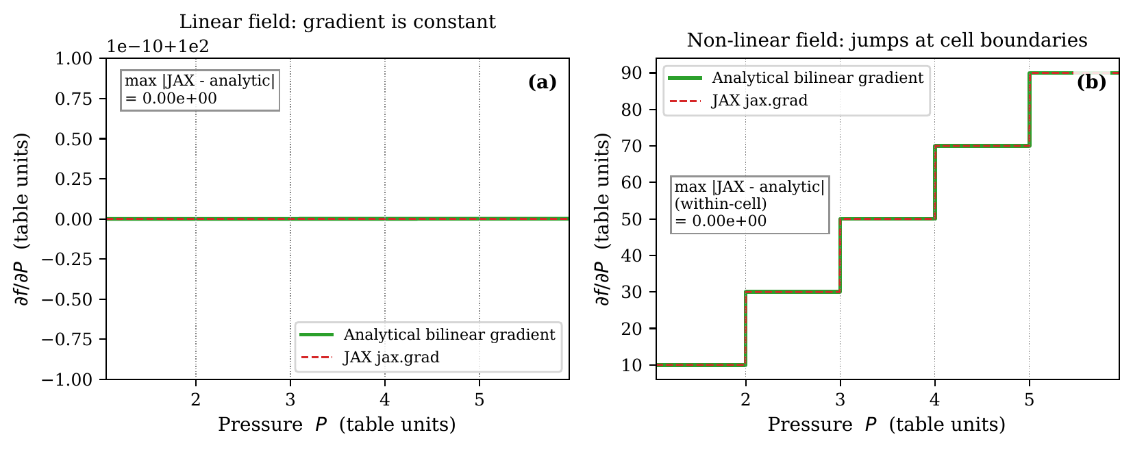
Figure 1. JAX-traced bilinear interpolation of the EOS table reproduces the numpy reference to float-64 machine precision and supplies finite, non-zero derivatives via jax.jacrev at on- and off-grid \((P, S)\) points. The agreement is the prerequisite for the analytic Jacobian path used by CVODE.

Phase evaluator tests

Test the SPIDER-parity behaviour of EntropyPhaseEvaluator:

• Phase identification at \((P, S)\) in pure solid, pure liquid, and mushy regimes.
• Viscosity tanh blend across the rheological transition \(\phi_\mathrm{rheo}\).
• Gravitational-separation velocity in viscous and inviscid regimes.
• Pressure-dependent latent heat \(L(P) = T_\mathrm{liq}(P) [S_\mathrm{liq}(P) - S_\mathrm{sol}(P)]\).

Solver integration tests

Drive EntropySolver through short integrations and check the resulting profiles:

• Standalone grey-body cooling: a fully-molten initial state cools toward the equilibrium temperature without status flag failures.
• The set_initial_entropy, set_initial_dSdr_cmb, and set_initial_core_temperature paths produce the expected state-vector layouts for quasi_steady, energy_balance, and bower2018 modes.
• The retry-ladder hooks (get_current_dSdr_cmb, _atol_sf) round-trip cleanly.

Conservation tests (tests/test_entropy_verification.py)

The conservation tests are the strongest class of verification because they hold under any valid run, not just specific test scenarios:

• Energy conservation. \(E_\mathrm{th}\) change over a closed integration matches the time-integrated surface flux to within solver tolerance.
• Mass conservation. Mantle mass remains constant through phase changes.
• Grey-body cooling. Surface flux follows \(\varepsilon\sigma(T_\mathrm{top}^4 - T_\mathrm{eqm}^4)\) within tolerance once the radiative regime is established.

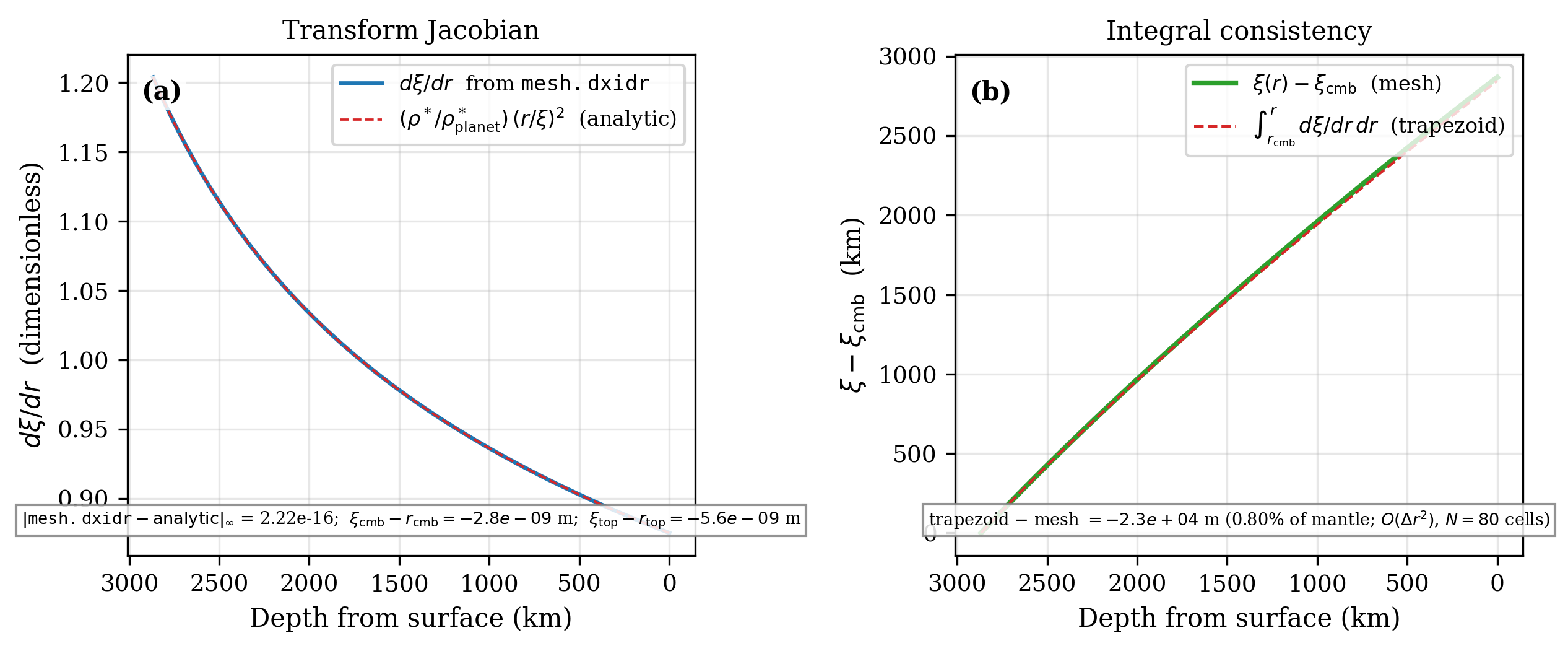
Figure 2. Mass-coordinate mesh Jacobian. The Newton solve that maps from mass coordinate to spatial radius (used when mass_coordinates = true) is monotone, smooth, and consistent with the analytic Adams-Williamson density profile. Departures here would propagate to mis-aligned cell volumes and a spurious mass-conservation residual in the integrator.

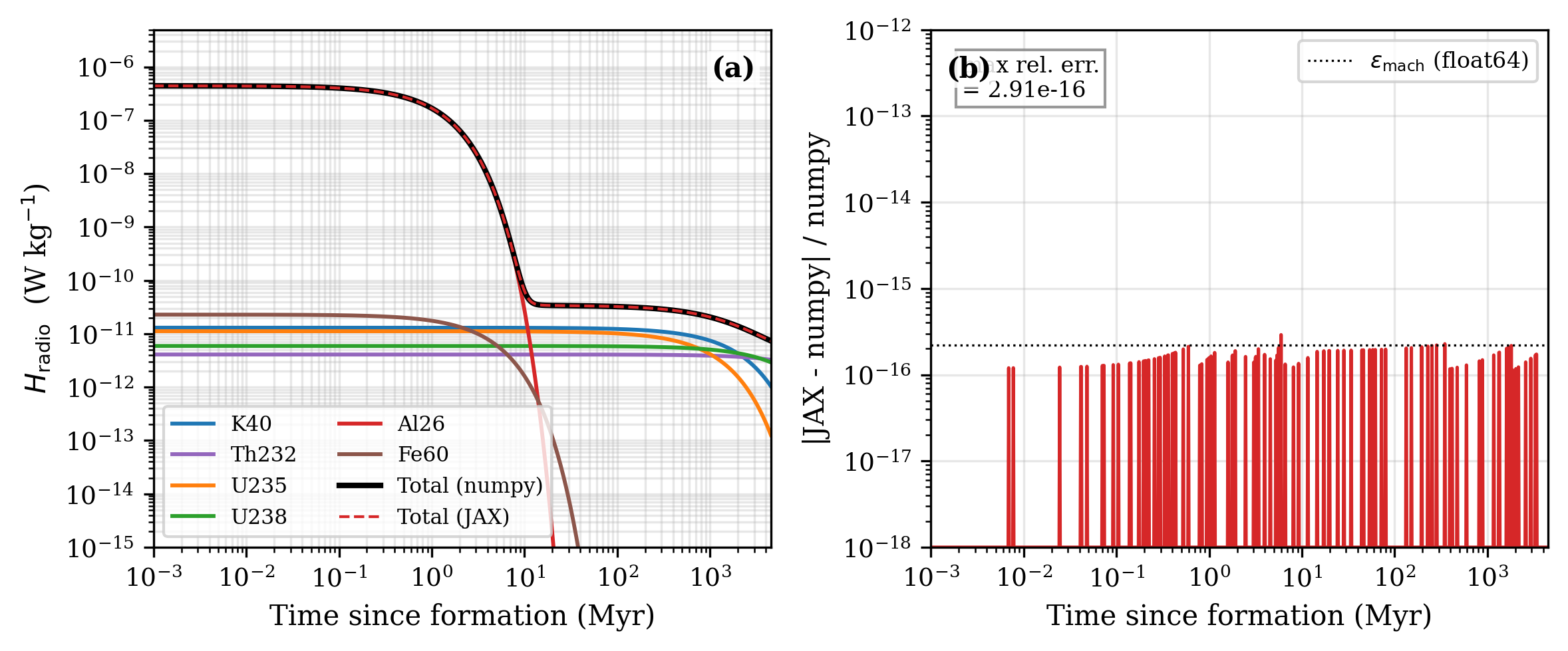
Figure 3. Radioactive heating \(H_\mathrm{radio}(t)\) for the bundled isotope cocktail (Ruedas 2017): present-day specific powers (\(^{40}\mathrm{K}\), \(^{232}\mathrm{Th}\), \(^{235}\mathrm{U}\), \(^{238}\mathrm{U}\)) decayed back to Solar System formation. Used as the source-term verification for the closed-mantle energy balance: the cumulative step_dE_Q_radio_J integral must match the time integral of \(\rho \cdot H_\mathrm{radio}\) over each call to within solver tolerance.

JAX path tests (tests/test_jax_entropy.py)

Verify that the JAX-backed EntropyEOS_JAX and compute_fluxes agree with the numpy path:

• EOS parity: EntropyEOS_JAX returns the same temperature, density, heat capacity, thermal expansivity, \(\partial T/\partial P|_S\), and conductivity as EntropyEOS on the same \((P, S)\) inputs.
• Phase evaluator parity: the JAX two-stage blend matches EntropyPhaseEvaluator to within floating-point tolerance.
• JIT and vmap compatibility: the JAX flux assembly is differentiable end-to-end with jax.grad/jax.jacrev and survives JIT compilation without recompilation hot-spots.
• Boundary-copy tests: dSdr boundary values copy from the nearest interior node (SPIDER ic.c:450 parity) instead of being extrapolated.
• Solver parity: integrating the same problem with the JAX-RHS-driven CVODE path and the numpy RHS produces matching trajectories.

Numpy ↔ JAX RHS parity at representative magma-ocean states

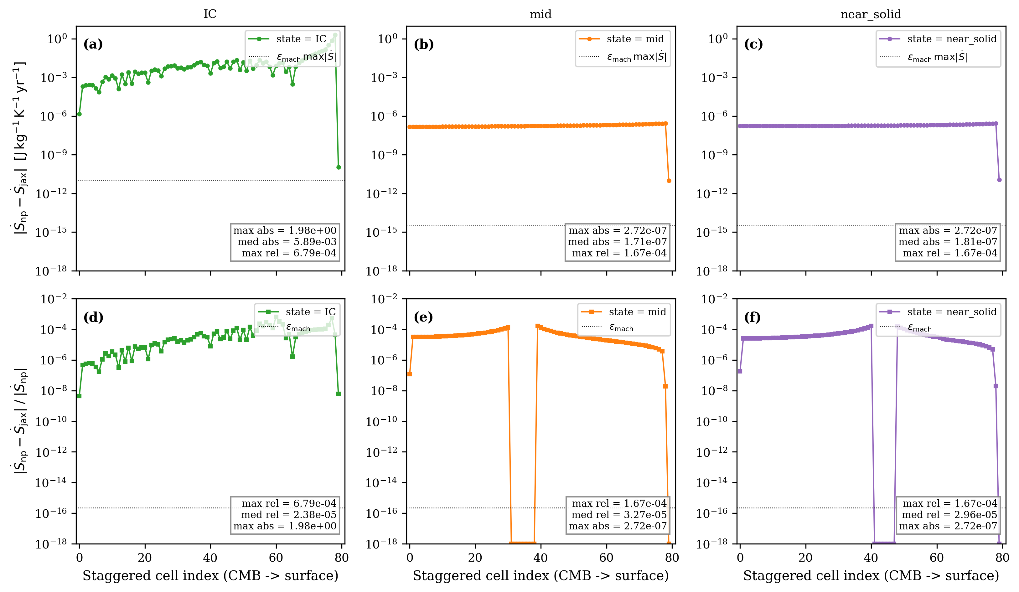
Figure 4. Numpy \(\leftrightarrow\) JAX RHS parity on an 80-cell Earth mesh at three representative magma-ocean states. Top row, panels (a-c): per-cell absolute residual \(|\dot S_\text{numpy} - \dot S_\text{jax}|\) in J/kg/K/yr; the dotted line is \(\epsilon_\mathrm{mach}\,\max|\dot S|\) (the floating-point round-off floor expected on a single FP operation). Bottom row, panels (d-f): per-cell relative residual \(|\dot S_\text{numpy} - \dot S_\text{jax}|/|\dot S_\text{numpy}|\); the dotted line is float-64 machine epsilon. The three states are (a/d) initial condition (full magma ocean, \(S \approx 3900\) J/kg/K, dimensionally uniform), (b/e) mid-solidification (\(S = 3300 \to 3700\) J/kg/K from CMB to surface), (c/f) near-solid (\(S = 3000 \to 3300\) J/kg/K).

Per-panel residuals:

• Mid-solidification (b, e) and near-solid (c, f). Interior cells sit at the float-64 round-off floor. Maximum absolute residual \(\sim 3\times 10^{-7}\) J/kg/K/yr, dominated by a single spike at the surface boundary cell where the BC assembly is re-derived independently between numpy and JAX. Median relative error \(\le 3\times 10^{-5}\).
• Uniform-entropy IC (a, d). Absolute residual \(\sim 1\) J/kg/K/yr. Both paths run EOS lookup, lever-rule, and table interpolation on a uniform input; the arithmetic differs at the interpolation level. The relative error inflates because \(|\dot S|\) itself is small in equilibrium.

Numpy and JAX paths are independent re-derivations, not a bit-exact port.

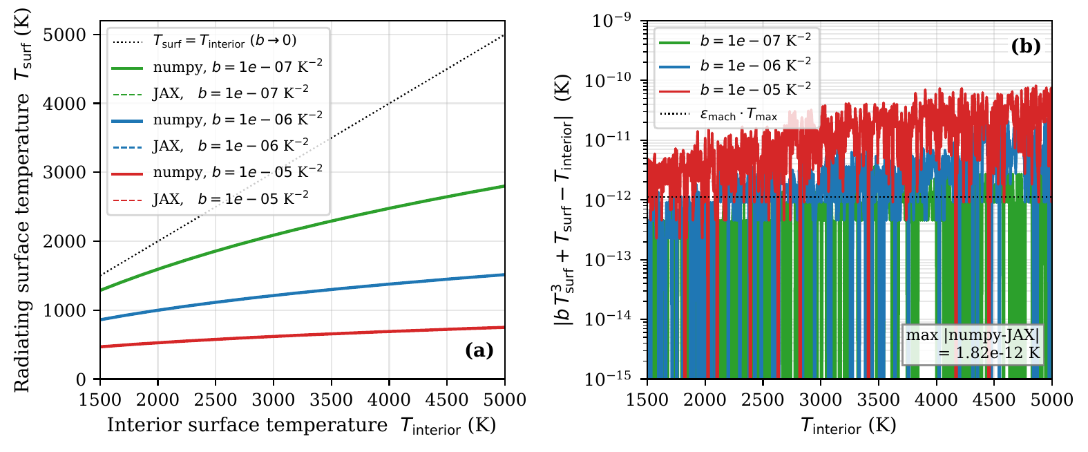
Figure 5. Surface-temperature correction from the upper-thermal-boundary-layer parameterisation (solver/boundary.py::_utbl_tsurf). The Cardano-formula solution to \(b x^3 + x - T_\mathrm{int} = 0\) recovers \(T_\mathrm{surf} < T_\mathrm{int}\) for the entire physical range and matches the cubic-equation residual to floating-point tolerance. Verifies the analytic surface boundary condition used when param_utbl = true.

Mesh tests (tests/test_jax_mesh_gravity_fallback.py)

Verify that when the external mesh file (eos_method = 2) supplies an eos_gravity column, the JAX path interpolates the per-node gravity profile onto the basic grid rather than broadcasting a single scalar.

Running the verification suite

The standalone suite uses pytest:

# Run the entire suite
pytest tests/

# Run a specific category
pytest tests/test_entropy_pytest.py
pytest tests/test_entropy_verification.py
pytest tests/test_jax_entropy.py

# Mark-filtered subsets
pytest -m unit tests/             # unit tests only
pytest -m smoke tests/            # smoke tests only

The JAX-path tests require jax and equinox to be installed; tests are skipped (not failed) when the optional dependencies are missing. Some tests also require the SPIDER-format EOS table directory; they skip if FWL_DATA is unset or does not contain the expected files.

Physical constraints checked

The suite asserts the following physical invariants on every solver-driven test run:

1. Temperature positivity. \(T > 0\) everywhere at all integration times. EOS lookups outside the table domain raise rather than silently extrapolating.
2. Melt fraction bounds. \(0 \le \phi \le 1\) via the smooth-clip; the assertion runs at every staggered node.
3. Pressure positivity and monotonicity. \(P(r)\) is positive and decreases monotonically from CMB to surface.
4. Entropy gradient continuity. \(\partial S/\partial r\) and the resulting fluxes are \(C^0\) across the solidus and liquidus crossings (the smoothing functions enforce this).
5. Energy conservation. Within the integrator tolerance, \(\Delta E_\mathrm{th}\) matches the time-integrated boundary fluxes plus internal heating sources.
6. Mass conservation. Total mantle mass is preserved under gravitational separation and chemical mixing (the segregation flux is divergence-free in mass).