JANUS: Physical model overview
A 1D prescribed convective atmosphere model for rocky exoplanet and magma ocean atmospheres.
1. Model summary
JANUS computes the temperature-pressure (T–p) structure of a planetary atmosphere in hydrostatic and convective equilibrium, then calculates the resulting radiative energy fluxes. It is designed for atmospheres overlying magma ocean surfaces, where surface temperatures are high, atmospheric compositions are diverse and potentially non-dilute in condensable species, and the standard dilute-vapour approximations of terrestrial meteorology break down. The model operates as a 1D column, integrating upward from a prescribed surface temperature and set of volatile partial pressures 12.
2. Vertical coordinate and hydrostatic balance
The atmosphere is discretised on a pressure grid from the surface pressure \(p_s\) down to a top-of-atmosphere pressure \(p_{\rm top}\) (typically \(10^{-5}\) bar). The geometric altitude \(z\) at each level is obtained from the hydrostatic equation combined with the ideal gas equation of state:
where \(\mu\) is the local mean molar mass of the gas mixture, \(g\) is the local gravitational acceleration, \(R = 8.3145\) J mol\(^{-1}\) K\(^{-1}\) is the universal gas constant, and \(T\) is the local temperature. Gravity varies with height:
where \(g_s = GM_p / r_p^2\) is the surface gravity, \(M_p\) the planetary mass, and \(r_p\) the planetary radius. Equation (1) is integrated upward using a forward Euler step, giving altitude from pressure differences. Note that this integration is used only to compute the diagnostic altitude grid — the T–p profile itself is integrated directly in pressure space using the pseudoadiabat ODE (Section 3.2).
3. Temperature-pressure profile
3.1 Dry adiabat
In regions where no volatile species condense, the temperature follows the dry adiabat:
where \(c_p^{\rm mix}\) is the molar heat capacity of the local gas mixture. The adiabatic exponent \(R/c_p^{\rm mix}\) is computed from the molar-weighted heat capacities of all species present.
3.2 Heat capacities
Gas-phase molar heat capacities are temperature-dependent, computed from Shomate polynomials 1:
where \(\hat T = T/1000\) and the fit constants \(A_s\)–\(E_s\) are taken from the NIST Chemistry WebBook (SRD 69).
3.3 Generalised moist pseudoadiabat
When one or more volatile species reach their saturation vapour pressure, the atmosphere becomes convectively unstable and the temperature-pressure slope is set by the generalised multi-species pseudoadiabat 3. This generalises the single-species derivation of Pierrehumbert (2010) 4 to \(N\) condensing species of arbitrary concentration and a freely tunable retained condensate fraction \(f_c \in [0,1]\).
The lapse rate is computed in two steps. First, the slope with respect to the dry partial pressure \(p_d\) (Graham et al. 2021 3 Eq. 15):
where \(\eta_s = x_s^{\rm gas} / x_d\) is the ratio of the gas-phase mole fraction of condensable \(s\) to the total dry mole fraction, \(\eta_s^c = x_s^{\rm cond} / x_d\) is the condensate mole fraction normalised by the dry mole fraction, \(L_s\) is the molar latent heat, \(c_{p,s}\) is the molar heat capacity of species \(s\) in the gas phase, \(c_{p,s}^{\rm cond}\) is the heat capacity of the condensed phase, \(\beta_s = L_s / (R T)\) is the dimensionless latent heat parameter, and \(f_c\) is the retained condensate fraction 3.
Second, this is converted to the total pressure gradient via the chain rule (Graham et al. 2021 3 Eq. 16):
where
This ODE in \((\ln p, \ln T)\) space is integrated upward from the surface using a fourth-order Runge-Kutta scheme with step size \(\Delta \ln p = -0.01\) 3.
The parameter \(f_c = 0\) recovers the pure pseudoadiabatic limit (all condensate immediately rained out), while \(f_c = 1\) gives fully reversible adiabatic ascent (all condensate retained) 3.
3.4 Saturation vapour pressure and condensation
A species \(s\) is condensing at pressure level \(p\) when its partial pressure \(p_s \geq p_{\rm sat,s}(T)\). The saturation vapour pressure is computed from the integrated Clausius-Clapeyron equation anchored at the triple point 4:
switching between \(L_{\rm sublimation}\) below the triple point and \(L_{\rm vaporization}\) above it. For water, a lookup table is available, providing temperature-dependent \(L_{\rm vap}(T)\) and \(p_{\rm sat}(T)\) from the triple point (273.16 K) to the critical point (647.10 K).
Above the critical temperature, \(L_s = 0\): species become supercritical and are treated as permanently gaseous with no latent heat contribution to the lapse rate.
H\(_2\) is hardcoded as non-condensing at all temperatures relevant to magma ocean atmospheres (\(p_{\rm sat} \to 10^{30}\) Pa), reflecting the fact that H\(_2\) condensation occurs only below \(\sim 30\) K.
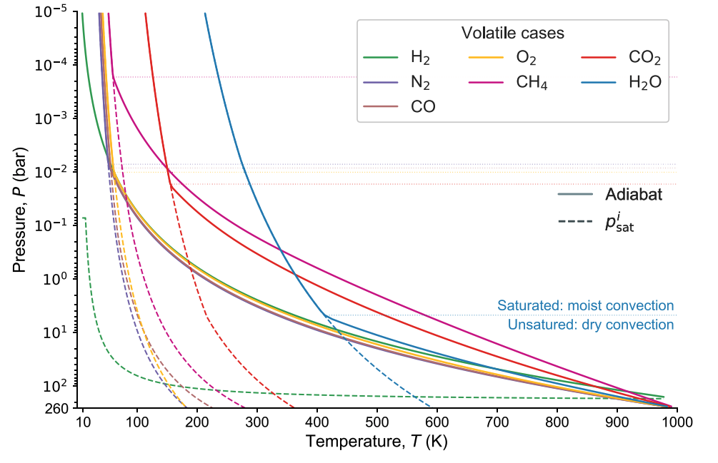
Thermal structure for single-species atmospheres with fixed surface pressure \(P_{\rm surf} = 260\) bar and surface temperature \(T_{\rm surf} = 1000\) K. Solid lines show the generalised adiabatic temperature profile (Eqs. 5–7) for each volatile; dashed lines show the corresponding saturation vapour pressure curve \(p_{\rm sat}^i\) (Eq. 8). In the lower troposphere the profile follows the dry adiabat until it intersects \(p_{\rm sat}^i\), at which point the lapse rate transitions to moist convection. Figure 3 from Lichtenberg et al. (2021) 1.
3.5 Condensate tracking
At each level, gas-phase and condensed-phase mole fractions are tracked separately:
- \(x_s^{\rm gas}\): mole fraction of species \(s\) in the gas phase
- \(x_s^{\rm cond}\): mole fraction of species \(s\) in the condensed phase
- \(x_d = \sum_{s \in \rm dry} x_s^{\rm gas}\): total dry gas mole fraction
- \(x_v = \sum_{s \in \rm wet} x_s^{\rm gas}\): total condensable vapour mole fraction
- \(x_c = \sum_s x_s^{\rm cond}\): total condensate mole fraction
The mean molar mass and heat capacity are updated at each level from these quantities. All condensate is assumed to be instantaneously rained out (for \(f_c = 0\)) and re-evaporated in sub-saturated regions at higher pressures.
4. Stratosphere
Above the tropopause, the atmosphere is set to an isothermal stratosphere at temperature \(T_r\). The stratosphere temperature is set to the radiative skin temperature 2 Eq. (8):
where \(\alpha_b\) is the Bond albedo, \(f_s\) is the instellation scaling factor, \(F_\star\) is the bolometric stellar flux, and \(\sigma_{\rm SB}\) is the Stefan–Boltzmann constant 4.
The tropopause is located by either a fixed temperature criterion, the first level where \(T \leq T_r\), or a heating rate criterion, where the tropopause is placed where the net radiative heating rate changes sign. In the stratosphere, volatile mixing ratios are fixed to their tropopause values.
Note
Setting \(T_r = 0\) K disables the stratosphere entirely: since no atmospheric
level reaches 0 K, the fixed-temperature criterion is never triggered and the
whole column is treated as convective. This is the appropriate choice for pure
steam atmospheres, and is the default in config_runaway.toml.
5. Radiative transfer
Radiative fluxes are computed by the SOCRATES radiative transfer suite 5, which solves the plane-parallel two-stream equations under the correlated-\(k\) approximation, using the random overlap method for combined gaseous absorption 2.
5.1 Thermal (longwave) fluxes
The upward and downward longwave fluxes satisfy the two-stream equation 1 Eq. (14):
with diffusivity factor \(D = 1.66\), optical depth \(\tau\), and Planck intensity \(B(T)\). The optical depth in differential form is 1 Eq. (19):
with mass mixing ratio \(\zeta_i\) and mass absorption coefficient \(k^i_\rho\) for species \(i\). The atmospheric heating rate is 1 Eq. (20):
with gravitational acceleration \(g\) and mean molecular weight \(\bar{\mu}_{\rm atm}\). The OLR is the upward thermal flux at the top of atmosphere:
5.2 Stellar (shortwave) flux
The absorbed stellar flux (ASF) at the top of atmosphere is 2:
where \(F_\star\) is the instellation, \(f_s = 3/8\) is an axial rotation scaling factor 6, \(\alpha_p\) is the planetary albedo, and \(\theta = 54.74°\) (\(= \arccos(1/\sqrt{3})\)) is the mean solar zenith angle 7.
5.3 Surface emission
The spectral surface emission in each SOCRATES band \(b\) is computed from the Planck function at wavenumber \(\tilde\nu_b\) (cm\(^{-1}\)):
with radiation constants \(c_1 = 1.191042 \times 10^{-5}\) and \(c_2 = 1.4387752\) (CGS wavenumber units), and surface albedo \(\alpha_{\rm surf}\).
5.4 Energy balance
The total upward and downward fluxes are the sum of thermal and stellar components 1 Eq. (17):
The net radiative flux used as the interior–atmosphere boundary condition is 1 Eq. (18), 2 Eq. (4):
Positive \(F_{\rm net}\) indicates the atmosphere is losing energy (cooling); negative indicates heating.
6. Coupled interior-atmosphere boundary condition
When coupled to an interior model, JANUS finds the surface temperature \(T_s\) such that the conductive flux through the surface skin layer equals the net atmospheric flux 2:
where \(k_{\rm c}\) is the thermal conductivity and \(d_{\rm c}\) the thickness of the conductive boundary layer. This root-finding problem is solved iteratively.
7. Runaway greenhouse physics
In a steam-dominated atmosphere, the OLR becomes decoupled from the surface temperature when the photosphere lies within a condensing region. Since the temperature structure in that region is fixed by the saturation curve rather than by \(T_s\), OLR saturates at the Simpson–Nakajima radiation limit (\(\approx 280\) W m\(^{-2}\) for pure steam) 8. Only when surface temperatures are high enough that the deep atmosphere becomes supercritical, and the condensing zone transparent, does the photosphere re-couple to \(T_s\), entering the post-runaway regime 9.
For multi-component outgassed atmospheres above molten surfaces, this classical radiation limit does not appear: the diverse gas mixture and volatile dissolution into the magma mean the OLR varies continuously with \(T_s\) with no clear plateau 10.
8. Rayleigh scattering
When enabled, Rayleigh scattering cross-sections are computed per spectral band and inserted into the SOCRATES spectral file at runtime. For CO\(_2\) and N\(_2\), the Vardavas & Carver (1984) 11 formula is used:
where \(\delta = (6 + 3\Delta)/(6 - 7\Delta)\) is the King factor, \(\Delta\) is the depolarisation ratio, \(A\) and \(B\) are species-specific refractivity coefficients from Allen's Astrophysical Quantities (2002), \(N_A\) is Avogadro's number, and \(\mu\) is the molar mass in kg mol\(^{-1}\).
For H\(_2\)O, a simpler \(\lambda^{-4}\) scaling is used instead, anchored to the mass-weighted cross-section at 1 μm from Pierrehumbert (2010) 4 Table 5.2:
where \(\sigma_{\rm 1\mu m} = 0.3743 \times 2.49 \times 10^{-6}\) m\(^2\) kg\(^{-1}\). Band-averaged coefficients are obtained by integrating over each spectral band and dividing by the band width.
9. Key model parameters and defaults
| Parameter | Symbol | Default | Notes |
|---|---|---|---|
| Retained condensate fraction | \(f_c\) | 0.0 | 0 = full rainout |
| Tropopause temperature | \(T_r\) | 0 K | 0 disables stratosphere |
| Mean zenith angle | \(\theta\) | 54.74° | Code default; Lichtenberg 2021 1 uses 54.55° |
| Bond albedo | \(\alpha_b\) | 0.175 | Applied before SOCRATES |
| Surface albedo | \(\alpha_{\rm surf}\) | 0.0 | Applied inside SOCRATES |
| Rotation scaling of instellation | \(f_s\) | 3/8 | Cronin (2014) 6 |
| Skin layer thickness | \(d_{\rm c}\) | 0.01 m | Used in coupled mode |
| Skin layer conductivity | \(k_{\rm c}\) | 2.0 W m\(^{-1}\) K\(^{-1}\) | Used in coupled mode |
| Gas overlap method | — | Random Overlap | SOCRATES overlap_type=2 |
| TOA pressure | \(p_{\rm top}\) | \(10^{-5}\) bar | User-configurable |
| RK4 step size | \(\Delta\ln p\) | −0.01 | Pseudoadiabat integration |
-
Lichtenberg, T., Bower, D. J., Hammond, M., Boukrouche, R., Sanan, P., Tsai, S. M., & Pierrehumbert, R. T. (2021). Vertically resolved magma ocean–protoatmosphere evolution: H₂, H₂O, CO₂, CH₄, CO, O₂, and N₂ as primary absorbers. Journal of Geophysical Research: Planets, 126(2), e2020JE006711. https://doi.org/10.1029/2020JE006711 ↩↩↩↩↩↩↩↩↩↩
-
Nicholls, H., Lichtenberg, T., Bower, D. J., & Pierrehumbert, R. (2024). Magma ocean evolution at arbitrary redox state. Journal of Geophysical Research: Planets, 129(12), e2024JE008576. https://doi.org/10.1029/2024JE008576 ↩↩↩↩↩↩
-
Graham, R. J., Lichtenberg, T., Boukrouche, R., & Pierrehumbert, R. T. (2021). A multispecies pseudoadiabat for simulating condensable-rich exoplanet atmospheres. The Planetary Science Journal, 2(5), 207. https://doi.org/10.3847/PSJ/ac214c ↩↩↩↩↩↩
-
Pierrehumbert, R. T. (2010). Principles of Planetary Climate. Cambridge University Press. ↩↩↩↩
-
Edwards, J. M., & Slingo, A. (1996). Studies with a flexible new radiation code. I: Choosing a configuration for a large-scale model. Quarterly Journal of the Royal Meteorological Society, 122(531), 689–719. https://doi.org/10.1002/qj.49712253107 ↩
-
Cronin, T. W. (2014). On the choice of average solar zenith angle. Journal of the Atmospheric Sciences, 71(8), 2994–3003. https://doi.org/10.1175/JAS-D-13-0392.1 ↩↩
-
Hamano, K., Kawahara, H., Abe, Y., Onishi, M., & Hashimoto, G. L. (2015). Lifetime and spectral evolution of a magma ocean with a steam atmosphere. The Astrophysical Journal, 806(2), 216. https://doi.org/10.1088/0004-637X/806/2/216 ↩
-
Nakajima, S., Hayashi, Y. Y., & Abe, Y. (1992). A study on the runaway greenhouse effect with a one-dimensional radiative-convective equilibrium model. Journal of the Atmospheric Sciences, 49(23), 2256–2266. https://doi.org/10.1175/1520-0469(1992)049 ↩
-
Boukrouche, R., Lichtenberg, T., & Pierrehumbert, R. T. (2021). Beyond runaway: initiation of the post-runaway greenhouse state on rocky exoplanets. The Astrophysical Journal, 919(2), 130. https://doi.org/10.3847/1538-4357/ac1345 ↩
-
Boer, I. D., Nicholls, H., & Lichtenberg, T. (2025). Absence of a runaway greenhouse limit on lava planets. The Astrophysical Journal, 987(2), 172. https://doi.org/10.3847/1538-4357/add69f ↩
-
Vardavas, I. M., & Carver, J. H. (1984). Solar and terrestrial parameterizations for radiative-convective models. Planetary and Space Science, 32(10), 1307–1325. https://doi.org/10.1016/0032-0633(84)90074-6 ↩