Dispatching an escape regime

The first run applied one prescription, energy-limited escape, to every state. This tutorial uses the regime dispatcher instead. You give zephyrus.dispatch one planetary state. It decides which escape physics applies to that state and returns the rate that physics gives, split over elements, together with flags and diagnostics that say how close the state sat to each regime boundary.

The escape regimes page explains the physics behind every step. This page shows how to drive it.

Before you start

The tutorial is one script, examples/demo_dispatcher/demo_dispatcher.py, and every code block on this page is a section of it, included verbatim. The script is not part of the installed package, so you need a clone of the repository:

git clone https://github.com/FormingWorlds/ZEPHYRUS.git
cd ZEPHYRUS
pip install -e .

Step 7 also needs the MORS stellar tracks: set FWL_DATA and run mors download all (see the installation guide).

There are two ways to follow along:

• Run the whole script from the repository root with python examples/demo_dispatcher/demo_dispatcher.py. It prints each step's output under a header such as === Step 3: ... === and writes both figures to output/. It takes about ten seconds.
• Or open a Python session (python or ipython) at the repository root and paste the blocks in page order. Each block uses names defined by the blocks above it, so do not skip one.

Every output shown below is what the script prints. Your last digit may differ between platforms.

The first block imports what the tutorial needs:

import dataclasses
import math
import os

import mors
import numpy as np
from scipy.constants import Stefan_Boltzmann as SIGMA_SB

from zephyrus import plot
from zephyrus.composition import atomize, species_mass_amu
from zephyrus.constants import au2m, rate_floor, yr_julian
from zephyrus.dispatcher import DispatchSettings, EscapeInputs, dispatch
from zephyrus.planets_parameters import Ls, Me, Me_atm, Ms, Re
from zephyrus.profiles import isothermal_profile

os.makedirs('output', exist_ok=True)
plot.apply_theme()  # PROTEUS figure style, when proteus-mpl is installed

plot.apply_theme() applies the PROTEUS figure style when the optional proteus-mpl package is installed, and does nothing otherwise.

Step 1: build a planetary state

The energy-limited function takes scalars only. The dispatcher also needs the structure of the atmosphere, because the quantities that decide the regime are found at different heights in it:

• The wind base, the pressure level where stellar XUV photons are absorbed and a wind would be launched.
• The sonic point, where such a wind reaches the speed of sound.
• The exobase, above which particles rarely collide and escape one at a time.

A state is therefore a set of scalars plus a Profile of pressure, temperature, radius, and composition. build_state assembles one, and every later step calls it:

print('=== Step 1: build a planetary state ===')

A_REF = 0.0775 * au2m  # orbit where a Sun-like star gives T_eq = 1000 K  [m]
P_SURF, P_TOP = 1.0e7, 1.0e-5  # profile from 100 bar up to 0.1 nbar      [Pa]

COMPOSITIONS = {  # mole fractions, the same at every level
    'CO2': {'CO2': 1.0},
    'N2-O2': {'N2': 0.8, 'O2': 0.2},
    'H/He': {'H2': 0.9, 'He': 0.1},
    'CO2 + 1% H2': {'CO2': 0.99, 'H2': 0.01},
}


def build_state(composition, m_earth, r_earth, f_xuv, settings=None, a=A_REF, inventory=Me_atm):
    """Planet of m_earth Earth masses and r_earth Earth radii, isothermal atmosphere."""
    gas = COMPOSITIONS[composition]
    M_p, R_p = m_earth * Me, r_earth * Re
    T_eq = (Ls / (16.0 * math.pi * SIGMA_SB * a**2)) ** 0.25  # zero albedo  [K]
    elements = atomize(gas)  # mole fraction of each element
    norm = sum(x * species_mass_amu(el) for el, x in elements.items())
    return EscapeInputs(
        M_p=M_p,  # planet mass                       [kg]
        R_p=R_p,  # planet radius                     [m]
        M_star=Ms,  # stellar mass                    [kg]
        a=a,  # semi-major axis                       [m]
        e=0.0,  # eccentricity
        T_eq=T_eq,  # equilibrium temperature         [K]
        F_xuv=f_xuv,  # XUV flux at the planet        [W m-2]
        F_bol=Ls / (4.0 * math.pi * a**2),  # bolometric flux  [W m-2]
        F_int=1.0,  # interior heat flux              [W m-2]
        kappa_photo=0.01,  # photospheric opacity     [m2 kg-1]
        profile=isothermal_profile(M_p, R_p, T_eq, gas, P_SURF, P_TOP),
        settings=settings or DispatchSettings(),
        age=1.0e8 * yr_julian,  # age of the snapshot, 100 Myr  [s]
        reservoirs={  # element inventories             [kg]
            el: inventory * x * species_mass_amu(el) / norm for el, x in elements.items()
        },
    )


state = build_state('CO2', 1.0, 1.0, 10.0)
profile = state.profile
print(f'T_eq        {state.T_eq:.1f} K')
print(f'F_bol       {state.F_bol:.4g} W m-2')
print(f'levels      {profile.p.size}, from {profile.p[0]:.3g} to {profile.p[-1]:.3g} Pa')
print(f'radius      {profile.r[0] / Re:.3f} to {profile.r[-1] / Re:.3f} Earth radii')
print(f'reservoirs  {", ".join(f"{el} {m:.4g} kg" for el, m in state.reservoirs.items())}')

=== Step 1: build a planetary state ===
T_eq        999.8 K
F_bol       2.266e+05 W m-2
levels      120, from 1e+07 to 1e-05 Pa
radius      1.000 to 1.091 Earth radii
reservoirs  C 1.406e+18 kg, O 3.744e+18 kg

In a coupled run the atmosphere module supplies the profile. Here isothermal_profile builds an isothermal atmosphere in hydrostatic balance, at the equilibrium temperature, from \(100\,\mathrm{bar}\) up to \(0.1\,\mathrm{nbar}\). That is crude, but it is enough to reach every branch of the dispatcher. Four choices in build_state change results, not only labels:

• The top pressure, \(0.1\,\mathrm{nbar}\). The XUV wind base sits near \(1\,\mathrm{nbar}\) for hydrogen and at a few tens of nanobar for carbon dioxide (\(33\,\mathrm{nbar}\) on this planet, step 5). If the profile stops below the wind base, the code clamps the base: a clamp, in the code's terms, replaces a value outside the range the code can evaluate with the nearest value inside it. Here the base would be placed at the profile top, and the flags base_clamped and base_clamp_decades would report it and how many decades of pressure it moved.
• The photospheric opacity, \(0.01\,\mathrm{m^2\,kg^{-1}}\). It sets the level the boil-off outflow of step 4 starts from, and the boil-off rate scales as its inverse. The value is a typical grey opacity, not a computed one. A coupled run should pass the mean opacity that the atmosphere model (AGNI, in PROTEUS) finds at the photospheric level.
• The orbit. At \(0.0775\,\mathrm{au}\) from a star of one solar luminosity, the equilibrium temperature is \(1000\,\mathrm{K}\). Deriving the temperature and the bolometric flux from the orbit keeps the three consistent.
• The interior heat flux, \(1\,\mathrm{W\,m^{-2}}\). With the default settings it reaches only the diagnostics (step 4 explains when it can set the rate).

The age and the element inventories (reservoirs, here one Earth atmosphere of \(\mathrm{CO_2}\) by mass) are optional. Supply them anyway: the diagnostics use them to check whether the rate could have been sustained for that long (step 5).

Step 2: dispatch one state and read the result

Dispatch the carbon dioxide planet of step 1, with \(1\,M_\oplus\) and \(1\,R_\oplus\), at an XUV flux of \(10\,\mathrm{W\,m^{-2}}\):

print('=== Step 2: dispatch one state and read the result ===')

result = dispatch(state)
total = sum(result.per_species.values())

print(f'regime       {result.regime}')
print(f'mdot         {result.mdot:.4e} kg/s')
for element, rate in result.per_species.items():
    print(f'  {element:<10} {rate:.4e} kg/s')
print(f'closure      {abs(total / result.mdot - 1.0) < 1e-12}')
print(f'flags        {result.flags}')
print(f'diagnostics  {len(result.diagnostics)} groups')

=== Step 2: dispatch one state and read the result ===
regime       hydrodynamic:EL
mdot         2.3477e+06 kg/s
  C          6.6130e+05 kg/s
  O          1.6864e+06 kg/s
closure      True
flags        {}
diagnostics  19 groups

The result has five fields:

• regime is one of six labels, listed in the results reference. Here it is hydrodynamic:EL: a fluid wind whose rate is set by the energy-limited formula.
• mdot is the bulk mass-loss rate in \(\mathrm{kg\,s^{-1}}\), never negative.
• per_species splits that rate over elements. The element rates add up to mdot to machine precision, which a coupled run relies on when it removes mass from each element's inventory. The closure line checks it.
• flags records every clamp (defined in step 1), fallback, or warning that fired. Empty means nothing needed reporting.
• diagnostics holds the supporting numbers that step 5 reads.

dispatch raises ValueError only for malformed input, such as a negative mass or a pressure profile that increases with height. Any physically posed state returns a result, however extreme.

Step 3: sweep the XUV flux across two regime boundaries

A star's XUV output falls by orders of magnitude as it ages, so a sweep in flux at a fixed orbit shows what happens to the planet as its star ages. Dispatch the same planet at 30 fluxes, for two compositions, and print every third \(\mathrm{CO_2}\) result:

print('=== Step 3: sweep the XUV flux across two regime boundaries ===')

fluxes = np.logspace(-2, math.log10(5.0e3), 30)  # [W m-2]
sweeps = {
    composition: [dispatch(build_state(composition, 1.0, 1.0, f)) for f in fluxes]
    for composition in ('CO2', 'N2-O2')
}

print(
    f'{"F_xuv [W m-2]":>13}  {"regime":<16} {"mdot [kg/s]":>11}  {"Kn_sc":>8}  '
    'label at Kn_crit 0.1 | 3'
)
for f_xuv, out in list(zip(fluxes, sweeps['CO2']))[::3]:
    kn = out.diagnostics['knudsen']
    edges = kn['counterfactual_labels']
    print(
        f'{f_xuv:13.3g}  {out.regime:<16} {out.mdot:11.3e}  {kn["kn_sc"]:8.3g}  '
        f'{edges[0.1]} | {edges[3.0]}'
    )

=== Step 3: sweep the XUV flux across two regime boundaries ===
F_xuv [W m-2]  regime           mdot [kg/s]     Kn_sc  label at Kn_crit 0.1 | 3
         0.01  hydrostatic       4.992e-123  8.99e+18  hydrostatic | hydrostatic
       0.0389  hydrostatic       4.992e-123  4.56e+18  hydrostatic | hydrostatic
        0.151  hydrostatic       4.992e-123       384  hydrostatic | hydrostatic
        0.587  hydrostatic       4.992e-123      2.55  hydrostatic | hydrodynamic:EL
         2.28  hydrodynamic:EL    5.356e+05     0.347  hydrostatic | hydrodynamic:EL
         8.87  hydrodynamic:EL    2.082e+06    0.0922  hydrodynamic:EL | hydrodynamic:EL
         34.5  hydrodynamic:EL    8.090e+06    0.0317  hydrodynamic:EL | hydrodynamic:EL
          134  hydrodynamic:RR    2.682e+07    0.0127  hydrodynamic:RR | hydrodynamic:RR
          520  hydrodynamic:RR    5.989e+07   0.00564  hydrodynamic:RR | hydrodynamic:RR
     2.02e+03  hydrodynamic:RR    1.256e+08   0.00268  hydrodynamic:RR | hydrodynamic:RR

The label changes twice. At low flux the planet is hydrostatic: there is no wind, and particles escape one at a time from the exobase (Jeans escape). Above about \(1\,\mathrm{W\,m^{-2}}\) it is a wind. At the highest fluxes the wind's rate is set by the recombination-limited formula (hydrodynamic:RR) instead of the energy-limited one.

The column Kn_sc is the Knudsen number at the sonic point: the mean free path of a particle divided by the local scale height. When it is small, particles collide often and the gas behaves as a fluid, so a wind can exist. The dispatcher calls the state a wind when Kn_sc is below the threshold kn_crit, which defaults to 1. The last column shows the label the state would get at kn_crit = 0.1 and 3, the edges of the threshold's physical range.

To find where each label changes, boundary_flux repeatedly halves a flux interval that brackets the change, until the interval is 0.001 dex wide:

def boundary_flux(composition, lo, hi, settings=None):
    """Flux [W m-2] between lo and hi where the label changes, to 0.001 dex."""

    def label(f_xuv):
        return dispatch(build_state(composition, 1.0, 1.0, f_xuv, settings)).regime

    first = label(lo)
    while math.log10(hi / lo) > 1.0e-3:  # halve the bracket in log flux
        mid = math.sqrt(lo * hi)
        lo, hi = (mid, hi) if label(mid) == first else (lo, mid)
    return math.sqrt(lo * hi)


boundaries = {
    'CO2': [boundary_flux('CO2', 0.1, 10.0), boundary_flux('CO2', 10.0, 2000.0)],
    'N2-O2': [boundary_flux('N2-O2', 0.01, 10.0)],
}
bands = {  # the wind boundary at the two edges of the Knudsen criterion
    composition: tuple(
        boundary_flux(composition, 0.01, 100.0, DispatchSettings(kn_crit=kn_crit))
        for kn_crit in (3.0, 0.1)
    )
    for composition in ('CO2', 'N2-O2')
}

for composition in ('CO2', 'N2-O2'):
    lo, hi = bands[composition]
    lowest = sweeps[composition][0]
    listed = ', '.join(f'{b:.3g}' for b in boundaries[composition])
    print(composition)
    print(f'  regime boundaries       {listed} W m-2')
    print(f'  wind onset band         {lo:.3g} to {hi:.3g} W m-2, a factor {hi / lo:.2g}')
    print(
        f'  rate at 0.01 W m-2      {lowest.mdot:.2e} kg/s, above the floor: '
        f'{lowest.diagnostics["rate_floor"]["above_floor"]}'
    )
print(f'rate floor (1 proton/yr)  {rate_floor:.2e} kg/s')

CO2
  regime boundaries       1.01, 86.6 W m-2
  wind onset band         0.542 to 8.07 W m-2, a factor 15
  rate at 0.01 W m-2      4.99e-123 kg/s, above the floor: False
N2-O2
  regime boundaries       0.412 W m-2
  wind onset band         0.204 to 1.95 W m-2, a factor 9.6
  rate at 0.01 W m-2      1.53e-71 kg/s, above the floor: False
rate floor (1 proton/yr)  5.30e-35 kg/s

On the \(\mathrm{CO_2}\) planet the wind sets in at \(1.01\,\mathrm{W\,m^{-2}}\), and the recombination-limited rate takes over at \(86.6\,\mathrm{W\,m^{-2}}\). The \(\mathrm{N_2}\) and \(\mathrm{O_2}\) planet of the same mass and radius starts its wind about 2.5 times lower, at \(0.412\,\mathrm{W\,m^{-2}}\), and never reaches the recombination-limited label in this range. Composition moves the boundaries, not only the rates.

The last block draws both sweeps:

panels = [
    dict(
        title=title,
        F_xuv=fluxes,
        mdot=[out.mdot for out in sweeps[composition]],
        regime=[out.regime for out in sweeps[composition]],
        boundaries=boundaries[composition],
        band=bands[composition],
    )
    for composition, title in (('CO2', 'CO$_2$'), ('N2-O2', 'N$_2$ and O$_2$'))
]
fig = plot.plot_regime_sweep(panels)
fig.savefig('output/dispatcher_regime_sweep.png')
fig.savefig('output/dispatcher_regime_sweep.pdf')

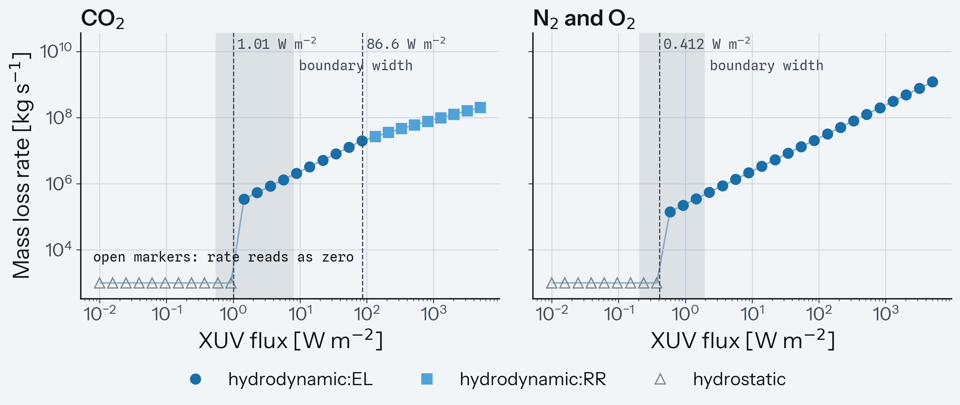
Two features of this figure matter.

The shaded band. Kinetic simulations place the transition from fluid to free particles at a Knudsen number near 0.1 when the heating is deposited in a thin layer, and near 1 when it is spread out¹. So the threshold has a physical range of 0.1 to 3, and the boundary it sets is a band rather than a line. On the \(\mathrm{CO_2}\) planet the wind sets in anywhere between \(0.542\) and \(8.07\,\mathrm{W\,m^{-2}}\), a factor of 15. Quote a regime boundary with this width. Every result already carries the labels at both edges, in diagnostics['knudsen']['counterfactual_labels'], so you do not need to rerun anything to find it.

The open markers. The hydrostatic rates, \(5.0 \times 10^{-123}\,\mathrm{kg\,s^{-1}}\) for \(\mathrm{CO_2}\) and \(1.5 \times 10^{-71}\,\mathrm{kg\,s^{-1}}\) for \(\mathrm{N_2}\) and \(\mathrm{O_2}\), are zero for any practical purpose. Two comparisons help you decide whether a rate matters:

• The rate floor, one proton mass per year (\(5.3 \times 10^{-35}\,\mathrm{kg\,s^{-1}}\)), is the smallest rate with physical meaning. diagnostics['rate_floor']['above_floor'] reports the comparison, and both rates fail it. The dispatcher never applies the floor itself: what counts as negligible is your decision.
• A rate above the floor can still be irrelevant. diagnostics['self_consistency'] compares the time to empty the inventory with the age of the state (step 5).

These rates vanish because heavy molecules on an Earth-mass planet are tightly bound at the exobase. The hydrostatic branch prescribes the exobase temperature, \(1000\,\mathrm{K}\) by default, and at that temperature a \(\mathrm{CO_2}\) molecule needs about 300 times its thermal energy to escape (step 5). Hydrostatic escape does real work where the gas is lighter, the planet smaller, or the exobase hotter: step 6 shows a Mars-mass planet with 1% hydrogen losing \(350\,\mathrm{kg\,s^{-1}}\) at the same default temperature.

Step 4: boil-off and Roche overflow

Two labels did not appear in the sweep, because neither depends on the XUV flux.

Boil-off. A hot, inflated hydrogen envelope can flow away on its own thermal energy, before stellar XUV matters. The dispatcher tests for this with the restricted Jeans parameter \(\Lambda\), the gravitational binding energy of a gas particle divided by its thermal energy, at the photosphere. Below a threshold of 20 the envelope boils off:

print('=== Step 4: boil-off and Roche overflow ===')

inflated = dispatch(build_state('H/He', 1.0, 1.5, 10.0))

print(f'regime     {inflated.regime}')
print(f'mdot       {inflated.mdot:.3e} kg/s')
print(f'Lambda     {inflated.diagnostics["lambda_gate"]:.3g}')
print(f'threshold  20, band {inflated.diagnostics["documentation"]["lambda_crit_band"]}')
print(f'flags      {sorted(inflated.flags)}')

=== Step 4: boil-off and Roche overflow ===
regime     boiloff
mdot       1.348e+14 kg/s
Lambda     2.89
threshold  20, band (15.0, 35.0)
flags      []

At \(1\,M_\oplus\) and \(1.5\,R_\oplus\), this hydrogen and helium envelope has \(\Lambda = 2.89\), far below 20, and loses \(1.3 \times 10^{14}\,\mathrm{kg\,s^{-1}}\). Boil-off is the regime of the first few million years, while young planets are still hot and inflated. The threshold itself has a literature range of 15 to 35, printed beside it.

No flag fires, although the XUV wind base was clamped: the isothermal envelope becomes unbound before it reaches \(1\,\mathrm{nbar}\), so the profile stops early and the base sits at the profile top. The boil-off outflow starts from the photosphere, not the wind base, so the clamp does not affect the rate, and the flags describe only what the dispatched rate depends on. diagnostics['base_level']['flags'] records the clamp on every call.

Roche overflow. A planet's gravity dominates the star's only out to the Hill radius. Gas that reaches beyond the Roche lobe, a smaller surface at about 0.70 Hill radii, is no longer bound to the planet. Take a puffier envelope, with \(3\,M_\oplus\) and \(1.7\,R_\oplus\), at \(0.1\,\mathrm{W\,m^{-2}}\). It has contracted just past the boil-off threshold. A boil-off outflow is still computed for it, with an upper limit set by the heat escaping from the planet's interior (the interior heat flux of step 1). An outflow sustained by that heat is core-powered mass loss (CPML)². Whether CPML continues once the envelope has contracted, with \(\Lambda\) above 20, is disputed. Gupta & Schlichting find that it persists for billions of years², while Tang et al. find that it removes at most 0.1% of the envelope once boil-off is modelled self-consistently³. By default the dispatcher therefore reports this outflow but does not let it compete for the rate. The residual_mode setting lets it compete:

admitted = DispatchSettings(residual_mode='luminosity_capped')
puffy = dispatch(build_state('H/He', 3.0, 1.7, 0.1, settings=admitted))
roche = puffy.diagnostics['roche']

print(f'regime            {puffy.regime}')
print(f'mdot              {puffy.mdot:.3e} kg/s, from the {roche["rate_branch"]} rate')
print(f'flow radius       {roche["flow_radius"] / roche["R_hill_periapsis"]:.3f} Hill radii')
print(
    f'atmosphere        {roche["r_atmosphere"] / puffy.diagnostics["nozzle"]["r_lobe"]:.3f} '
    f'Roche-lobe radii'
)
print(f'roche_subflag     {puffy.flags["roche_subflag"]}')

regime            roche_overflow
mdot              8.968e+06 kg/s, from the boiloff rate
flow radius       1.132 Hill radii
atmosphere        1.350 Roche-lobe radii
roche_subflag     dynamical

Admitted, this outflow wins, and its flow reaches 1.13 Hill radii. The dispatcher then renames the state roche_overflow. The rate is unchanged by the renaming: it is still the boil-off rate, which is why the output names that rate. Read it as a lower limit on what tides would remove. The subflag dynamical says the atmosphere itself extends past the Roche lobe, to 1.35 lobe radii. The troubleshooting guide explains the other subflag values.

Now dispatch the same state with the default settings:

default = dispatch(build_state('H/He', 3.0, 1.7, 0.1))
bolometric = default.diagnostics['bolometric']
nozzle = default.diagnostics['nozzle']

print(f'regime            {default.regime}')
print(f'mdot              {default.mdot:.3e} kg/s')
print(f'flow radius       {1.0 / default.diagnostics["roche"]["xi_flow"]:.3f} Hill radii')
print(f'flags             {sorted(default.flags)}')
print(
    f'bolometric        {bolometric["rate_kg_s"]:.3e} kg/s, competes: {bolometric["competes"]}'
)
print(
    f'L1 transfer       {nozzle["rate_full_orbit_kg_s"]:.3e} kg/s, competes: '
    f'{nozzle["rate_kg_s"] > 0.0} (R_sonic / R_L1 = {nozzle["R_sonic_over_R_L1"]:.3f})'
)

regime            hydrodynamic:PL
mdot              4.423e+04 kg/s
flow radius       0.817 Hill radii
flags             ['base_clamp_decades', 'base_clamped', 'near_roche', 'subcritical_sonic']
bolometric        8.968e+06 kg/s, competes: False
L1 transfer       6.749e+08 kg/s, competes: False (R_sonic / R_L1 = 0.957)

The XUV wind now sets the rate, at \(4.4 \times 10^{4}\,\mathrm{kg\,s^{-1}}\), two hundred times below the admitted outflow. The suffix PL means the rate is limited by the number of ionising photons arriving (step 6). The wind reaches 0.82 Hill radii. That is past the Roche lobe, at about 0.70 Hill radii, but the Roche-overflow label tests the flow radius against the Hill radius, not against the Roche lobe, so the state keeps its label and only the near_roche warning fires.

The last line is a third candidate. L1, the inner Lagrange point, is the point between planet and star where their gravity balances. Gas can flow through it towards the star as through a nozzle. The dispatcher computes that transfer rate on every call, here \(6.7 \times 10^{8}\,\mathrm{kg\,s^{-1}}\), but lets it compete only when the wind's sonic point reaches L1. Here the sonic point stops just short of it (R_sonic / R_L1 = 0.957), so a spherical wind forms first and the transfer rate does not count.

Step 5: read the diagnostics

The result of step 2 carries 19 groups of diagnostics. The dispatcher never reads them back when it decides, so they cannot change a verdict. They are there so you can judge how firm the verdict is. The results reference documents every key. This block reads the most useful ones for the \(\mathrm{CO_2}\) planet of step 2, in the order the questions usually come up:

print('=== Step 5: read the diagnostics ===')

d = result.diagnostics  # the carbon dioxide planet of step 2
kn, hydro = d['knudsen'], d['hydrodynamic']

print('Which branch, and how close was the switch?')
print(f'  Kn_sc {kn["kn_sc"]:.3g} against threshold {kn["threshold_applied"]:.3g}')
print(f'  label at the band edges: {kn["counterfactual_labels"]}')
print('What set the rate?')
print(f'  EL {hydro["mdot_el"]:.3e}, RR {hydro["mdot_rr"]:.3e}, PL {hydro["mdot_pl"]:.3e} kg/s')
print(
    f'  {hydro["selection_mechanism"]}, T_wind {hydro["T_wind"]:.0f} K, '
    f'barometric factor {hydro["rr_chain"]["barometric_factor"]:.2g}'
)
print('Could the heating drive a transonic flow?')
print(f'  Q_net / Q_c {d["johnson_q"]["q_net_over_qc"]:.3g}')
print('How does the verdict read in other classifications?')
guo = d['guo_triple']
print(
    f'  lambda_exo {guo["lambda_exo"]:.4g}, lambda_rp {guo["lambda_rp"]:.4g}, '
    f'lambda_star {guo["lambda_star"]:.4g}'
)
print(
    f'  log10(-phi) {d["potential_screens"]["log_minus_phi_cgs"]:.4g} (cgs), '
    f'Salz screen: {d["potential_screens"]["salz_verdict"]}'
)
print('Is the snapshot self-consistent?')
consistency = d['self_consistency']
print(f'  worst Kn below the sonic point {d["fluid_check"]["worst_kn"]:.3g}')
print(
    f'  inventory lasts {consistency["t_deplete_s"] / yr_julian:.3g} yr, '
    f'age {consistency["age_s"] / yr_julian:.3g} yr, '
    f'inconsistent: {consistency["inconsistent"]}'
)
print('Where was the wind launched, and where did the cross sections come from?')
print(
    f'  wind base {d["base_level"]["p_Pa"]:.3g} Pa, '
    f'clamped: {d["base_level"]["clamp_decades"] is not None}'
)
print(f'  cross sections: {kn["provenance"]}')

=== Step 5: read the diagnostics ===
Which branch, and how close was the switch?
  Kn_sc 0.0832 against threshold 1
  label at the band edges: {0.1: 'hydrodynamic:EL', 3.0: 'hydrodynamic:EL'}
What set the rate?
  EL 2.348e+06, RR 4.205e+06, PL 6.137e+06 kg/s
  EL-selected, T_wind 7903 K, barometric factor 0.0063
Could the heating drive a transonic flow?
  Q_net / Q_c 9.96
How does the verdict read in other classifications?
  lambda_exo 301.1, lambda_rp 330.9, lambda_star 303.6
  log10(-phi) 11.8 (cgs), Salz screen: wind
Is the snapshot self-consistent?
  worst Kn below the sonic point 0.124
  inventory lasts 6.95e+04 yr, age 1e+08 yr, inconsistent: True
Where was the wind launched, and where did the cross sections come from?
  wind base 0.00331 Pa, clamped: False
  cross sections: {'C': 'laricchiuta', 'O': 'laricchiuta'}

What each answer says:

• The switch. A Knudsen number of 0.083 is about 12 times below the threshold, and the label is the same at both edges of the band. A value within a few times of the threshold, or edge labels that differ, means the label depends on a choice within the criterion's range.
• The rate. The hydrodynamic wind rate is the smallest of three limits: energy-limited (EL), recombination-limited (RR), and photon-limited (PL). All three are computed, so you can see the margin. T_wind is the wind temperature set by the balance of heating and cooling, \(7903\,\mathrm{K}\) here. The barometric factor is the fraction of the gas density at the wind base that survives to the sonic point. When an RR rate wins, it tells you whether recombination at the base or the climb to the sonic point limited the wind (see the escape regimes page).
• The heating. \(Q_\mathrm{net}/Q_\mathrm{c}\) compares the absorbed heating with the power needed to drive a flow through the sonic point¹. Below 1, no wind is possible whatever a rate formula returns. At 10 there is an order of magnitude to spare.
• Other classifications. Papers classify escape with different quantities, and printing them lets a reader check the verdict in their own terms. Three are Jeans parameters, each the gravitational binding energy of a particle over its thermal energy, taken at a different place. lambda_exo is taken at the exobase with the exobase temperature, the form that sets the Jeans escape flux⁴. lambda_rp is taken at the planet radius with the equilibrium temperature, the restricted Jeans parameter of Fossati et al.⁵, here with the mean molecular mass as in Guo⁶. lambda_star is that parameter corrected for the star's tides, which Guo uses to tell thermally, tidally, and XUV-driven escape apart⁶. The gravitational potential, log10(-phi), is what Salz et al.⁷ use to separate winds from stable upper atmospheres. The exobase value of 301 is why the hydrostatic rates of step 3 vanish: the Jeans flux falls as \(e^{-301}\).
• Self-consistency. The fluid check reports the largest Knudsen number anywhere below the sonic point, 0.124. The inventory check is the sharp one: at this rate the planet empties one Earth atmosphere in \(7 \times 10^{4}\,\mathrm{yr}\), against the age of \(100\,\mathrm{Myr}\) supplied with the state. The state is valid input but cannot have lasted. A grid point that fails this check is a problem with the grid, not with the code.
• Provenance. The wind base was found inside the profile, so it was not clamped. The collision cross sections come from the tabulated collision integrals of Laricchiuta et al.⁸ for both elements. Where those tables lack a pair, a weaker fallback is used and named here.

Step 6: settings that move a boundary

All settings live in DispatchSettings and are listed in the parameter reference. This step varies five of them.

The Knudsen threshold

print('=== Step 6: settings that move a boundary ===')

for kn_crit in (0.1, 1.0, 3.0):
    out = dispatch(build_state('CO2', 1.0, 1.0, 2.0, DispatchSettings(kn_crit=kn_crit)))
    print(f'kn_crit {kn_crit:<4} at 2 W m-2: {out.regime}')

=== Step 6: settings that move a boundary ===
kn_crit 0.1  at 2 W m-2: hydrostatic
kn_crit 1.0  at 2 W m-2: hydrodynamic:EL
kn_crit 3.0  at 2 W m-2: hydrodynamic:EL

At \(2\,\mathrm{W\,m^{-2}}\) the \(\mathrm{CO_2}\) planet sits inside the band of step 3: hydrostatic at the strict edge, a wind at the default and at the lenient edge.

The exobase temperature

The hydrostatic branch does not compute the exobase temperature. It takes a prescribed value, T_exo_value, \(1000\,\mathrm{K}\) by default, and the Jeans flux depends on it exponentially. A Mars-mass planet (\(0.107\,M_\oplus\), \(0.53\,R_\oplus\)) with 1% hydrogen in its \(\mathrm{CO_2}\) shows what that does:

print(f'{"T_exo [K]":>9}  {"regime":<12} {"mdot [kg/s]":>11}  {"H [kg/s]":>9}  {"C [kg/s]":>9}')
for t_exo in (1000.0, 2000.0, 4000.0):
    settings = DispatchSettings(T_exo_value=t_exo)
    out = dispatch(build_state('CO2 + 1% H2', 0.107, 0.53, 0.01, settings))
    rates = out.per_species
    print(
        f'{t_exo:9.0f}  {out.regime:<12} {out.mdot:11.4g}  {rates["H"]:9.4g}  {rates["C"]:9.3g}'
    )

h2 = out.diagnostics['hydrostatic']['detail']['species']['H2']  # at 4000 K
print(
    f'H2 at 4000 K: lambda_exo {h2["lambda_exo"]:.3g}, '
    f'Jeans flux / diffusion supply {h2["phi_jeans"] / h2["phi_diffusion"]:.3g}'
)

T_exo [K]  regime       mdot [kg/s]   H [kg/s]   C [kg/s]
     1000  hydrostatic        346.9      346.9   7.76e-10
     2000  hydrostatic          353      352.8     0.0356
     4000  hydrostatic         1580      355.5        334
H2 at 4000 K: lambda_exo 0.282, Jeans flux / diffusion supply 56.7

From \(1000\) to \(4000\,\mathrm{K}\) the bulk rate rises by a factor of 4.6, while the carbon rate rises by more than 11 orders of magnitude. The two elements are limited differently. Hydrogen escapes easily (its exobase Jeans parameter is 0.28 at \(4000\,\mathrm{K}\)), and its Jeans flux is 57 times what diffusion through the \(\mathrm{CO_2}\) can supply from below. So the supply sets its rate, which changes by only 2.5% across the sweep. Carbon and oxygen are limited by the Jeans flux itself and carry the full exponential. The hydrostatic rate combines the two limits per species⁹, so a bulk rate can hide two very different mechanisms.

The sweep starts at \(1000\,\mathrm{K}\) because that is the temperature at the top of this profile. A lower prescription would describe an upper atmosphere that cools with height, so the dispatcher clamps it to the profile top temperature and flags it.

The heating efficiency and the three wind limits

The energy-limited rate assumes a fraction efficiency of the absorbed XUV energy lifts gas out of the planet's gravity well. The literature range is 0.1 to 0.6. Sweep it at two fluxes:

print(f'{"epsilon":>7}  {"F_xuv":>6}  {"regime":<16} {"EL":>9}  {"RR":>9}  {"PL":>9}  [kg/s]')
for eps in (0.1, 0.3, 0.6):
    for f_xuv in (3.0, 300.0):
        out = dispatch(build_state('CO2', 1.0, 1.0, f_xuv, DispatchSettings(efficiency=eps)))
        hy = out.diagnostics['hydrodynamic']
        print(
            f'{eps:7.1f}  {f_xuv:6.0f}  {out.regime:<16} {hy["mdot_el"]:9.3g}  '
            f'{hy["mdot_rr"]:9.3g}  {hy["mdot_pl"]:9.3g}'
        )
print(f'photon-limit efficiency {hy["efficiency_photon_limit"]:.3g}')

epsilon   F_xuv  regime                  EL         RR         PL  [kg/s]
    0.1       3  hydrodynamic:EL   7.04e+05   1.39e+06   1.84e+06
    0.1     300  hydrodynamic:RR   7.04e+07   4.36e+07   1.84e+08
    0.3       3  hydrodynamic:RR   2.11e+06   1.39e+06   1.84e+06
    0.3     300  hydrodynamic:RR   2.11e+08   4.36e+07   1.84e+08
    0.6       3  hydrodynamic:RR   4.23e+06   1.39e+06   1.84e+06
    0.6     300  hydrodynamic:RR   4.23e+08   4.36e+07   1.84e+08
photon-limit efficiency 0.261

The dispatched rate is the smallest of the three columns. At \(3\,\mathrm{W\,m^{-2}}\) and the default efficiency of 0.1, the energy limit is lowest. At 0.3 and above the recombination limit is lower, so more efficient heating cannot remove more gas and the rate stays at \(1.4 \times 10^{6}\,\mathrm{kg\,s^{-1}}\). The label changes although the wind itself does not. The photon limit would bind above an efficiency of 0.261: each ionising photon removes at most one particle, and lifting one particle out of the well of a \(1\,M_\oplus\) planet costs about a quarter of a photon's energy¹⁰. On this planet the recombination limit is lower still. On a hydrogen envelope, where a particle is far less tightly bound, the photon limit binds already at efficiencies of a few % (see the wind page).

Both the energy and photon limits are proportional to the flux. The recombination limit is not: a hundredfold rise in flux raises it only about 30 times. The base ion density follows the square root of the flux, and the wind also warms with flux, which lifts the rise from 10 to about 30. At \(300\,\mathrm{W\,m^{-2}}\) it is lowest at every efficiency, and the efficiency no longer matters. The settings photon_limit = False and recombination_limit = False remove the PL and RR limits, which reproduces codes that carry only the energy-limited formula.

Fractionation

In a wind, light elements can escape faster than heavy ones. The dispatcher solves for this with the closure on the fractionation page. Turning it off splits the rate by the inventory's mass fractions instead:

for fractionate in (True, False):
    out = dispatch(
        build_state('CO2', 1.0, 1.0, 10.0, DispatchSettings(fractionate=fractionate))
    )
    shares = {el: rate / out.mdot for el, rate in out.per_species.items()}
    print(
        f'fractionate {fractionate!s:<5}  '
        + ', '.join(f'{el} {s:.4f}' for el, s in shares.items())
    )

fractionate True   C 0.2817, O 0.7183
fractionate False  C 0.2729, O 0.7271

Carbon, the lighter element, is enriched by 3%. That is a small effect, as expected for a dense wind of heavy gas. On a hydrogen-rich atmosphere the difference is much larger, and it decides how the mean molecular weight of the atmosphere evolves.

Hysteresis, for time-stepping

A time-stepping run passes the previous result's rate_branch as prev_regime, and the dispatcher then shifts the Knudsen threshold to favour that branch. The branch is the label before any Roche renaming, so a wind renamed roche_overflow is still remembered as a wind. The shift is set by kn_hysteresis, a factor of 1.5 by default. After a hydrostatic step a wind needs Kn_sc below kn_crit / kn_hysteresis = 1 / 1.5 = 0.667, and after a wind step the wind persists until Kn_sc exceeds kn_crit * kn_hysteresis = 1.5. A track therefore cannot flip between branches on numerical noise:

print(f'{"F_xuv":>5}  {"previous label":<16} {"regime":<16} {"Kn_sc":>6}  threshold')
for f_xuv in (0.9, 1.1):
    for previous in (None, 'hydrostatic', 'hydrodynamic:EL'):
        hysteresis_state = build_state('CO2', 1.0, 1.0, f_xuv)
        hysteresis_state.prev_regime = previous
        out = dispatch(hysteresis_state)
        kn = out.diagnostics['knudsen']
        print(
            f'{f_xuv:5.2f}  {previous!s:<16} {out.regime:<16} {kn["kn_sc"]:6.3f}  '
            f'{kn["threshold_applied"]:.3g}'
        )

F_xuv  previous label   regime            Kn_sc  threshold
 0.90  None             hydrostatic       1.200  1
 0.90  hydrostatic      hydrostatic       1.200  0.667
 0.90  hydrodynamic:EL  hydrodynamic:EL   1.200  1.5
 1.10  None             hydrodynamic:EL   0.884  1
 1.10  hydrostatic      hydrostatic       0.884  0.667
 1.10  hydrodynamic:EL  hydrodynamic:EL   0.884  1.5

Inside the window the previous label is kept, in both directions. The threshold column shows when it was in use.

Step 7: follow a stellar XUV history

Load a MORS track for a Sun-like star, convert its luminosities to fluxes at \(0.2\,\mathrm{au}\), and dispatch one planet at 40 ages. The planet has \(1\,M_\oplus\) and \(1\,R_\oplus\), \(\mathrm{CO_2}\) with 1% hydrogen, and an inventory of 100 Earth atmospheres:

print('=== Step 7: follow a stellar XUV history ===')

A_TRACK = 0.2 * au2m  # [m]
star = mors.Star(Mstar=1.0, Omega=1.0)  # 1 solar mass, spinning at today's solar rate at 1 Myr
age_myr = np.asarray(star.Tracks['Age'])
l_xuv = (np.asarray(star.Tracks['Lx']) + np.asarray(star.Tracks['Leuv'])) * 1.0e-7  # erg/s to W
l_bol = np.asarray(star.Tracks['Lbol']) * 1.0e-7  # erg/s to W

# One frozen atmosphere with 100 Earth atmospheres of gas, at 40 ages along the track.
planet = build_state('CO2 + 1% H2', 1.0, 1.0, 0.0, a=A_TRACK, inventory=100.0 * Me_atm)
track, previous = [], None
for i in np.unique(np.linspace(0, age_myr.size - 1, 40).astype(int)):
    snapshot = dataclasses.replace(
        planet,
        T_eq=(l_bol[i] / (16.0 * math.pi * SIGMA_SB * A_TRACK**2)) ** 0.25,
        F_xuv=l_xuv[i] / (4.0 * math.pi * A_TRACK**2),
        F_bol=l_bol[i] / (4.0 * math.pi * A_TRACK**2),
        age=age_myr[i] * 1.0e6 * yr_julian,
        prev_regime=previous,
    )
    out = dispatch(snapshot)
    previous = out.rate_branch
    track.append(dict(age_myr=age_myr[i], F_xuv=snapshot.F_xuv, result=out))

print(
    f'{"age [Myr]":>9}  {"F_xuv":>6}  {"regime":<16} {"mdot [kg/s]":>11}  {"Kn_sc":>8}  '
    'consistent'
)
for row in track[::6]:
    out = row['result']
    print(
        f'{row["age_myr"]:9.1f}  {row["F_xuv"]:6.3g}  {out.regime:<16} {out.mdot:11.3e}  '
        f'{out.diagnostics["knudsen"]["kn_sc"]:8.3g}  '
        f'{not out.diagnostics["self_consistency"]["inconsistent"]}'
    )
for before, after in zip(track[:-1], track[1:]):
    if before['result'].regime != after['result'].regime:
        print(
            f'label changes between {before["age_myr"]:.0f} and {after["age_myr"]:.0f} Myr: '
            f'{before["result"].mdot:.3e} to {after["result"].mdot:.3e} kg/s'
        )

=== Step 7: follow a stellar XUV history ===
age [Myr]   F_xuv  regime           mdot [kg/s]     Kn_sc  consistent
      1.0    58.4  hydrodynamic:EL    1.274e+07     0.022  True
     45.0    1.62  hydrodynamic:EL    3.546e+05     0.543  True
    310.1     1.4  hydrodynamic:EL    3.048e+05     0.667  False
   1138.9   0.852  hydrodynamic:EL    1.860e+05      1.43  False
   3039.5   0.495  hydrostatic        4.902e-02      4.15  True
   6189.6    0.34  hydrostatic        4.902e-02      10.9  True
   9439.6   0.324  hydrostatic        4.902e-02      12.5  True
label changes between 1139 and 1369 Myr: 1.860e+05 to 4.902e-02 kg/s

The last block draws the track:

fig = plot.plot_track(
    age_myr=[row['age_myr'] for row in track],
    mdot=[row['result'].mdot for row in track],
    regimes=[row['result'].regime for row in track],
    per_species=[row['result'].per_species for row in track],
    inconsistent=[
        row['result'].diagnostics['self_consistency']['inconsistent'] for row in track
    ],
)
fig.savefig('output/dispatcher_track.png')
fig.savefig('output/dispatcher_track.pdf')

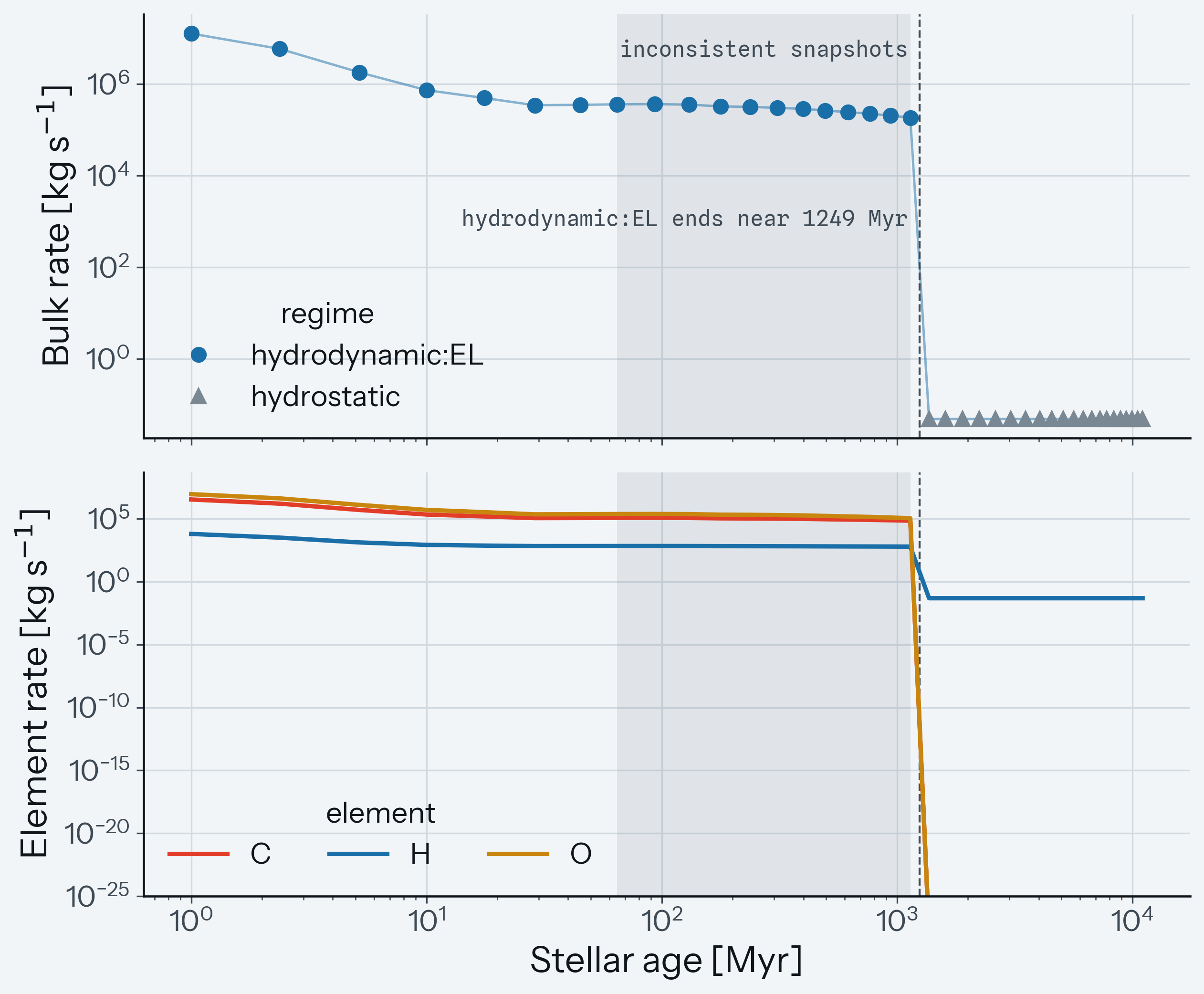
What the track shows:

• The label belongs to the state, not to the planet. Nothing about the planet changed. The star became quieter, the Knudsen number rose through the threshold, and near \(1.2\,\mathrm{Gyr}\) the escape changed from a wind to Jeans escape. At 1139 Myr the Knudsen number is already 1.43, and the wind holds because the previous step was a wind: that is the hysteresis window of step 6, which keeps it until the number passes 1.5.
• The rate drops by more than six orders of magnitude at the crossing, from \(1.9 \times 10^{5}\) to \(4.9 \times 10^{-2}\,\mathrm{kg\,s^{-1}}\). There is no smoothing between branches, so the size of this jump is a result you can quote. It measures how much the two descriptions disagree at the same state.
• What escapes changes too (lower panel). The wind carries carbon and oxygen away with the hydrogen. After the crossing hydrogen escapes alone, and the carbon and oxygen rates drop to about \(10^{-139}\,\mathrm{kg\,s^{-1}}\), off the bottom of the plot.
• The hydrostatic rate stays at \(4.9 \times 10^{-2}\,\mathrm{kg\,s^{-1}}\) for the remaining ten billion years. That branch contains no XUV physics: a prescribed exobase temperature, a frozen profile, and a diffusion-limited supply that does not see the star. The flat line shows what the branch leaves out. It is also why hydrostatic rates of heavy elements are flagged as lower limits: the non-thermal processes that remove heavy species from real upper atmospheres are not modelled.
• The consistency check fails between \(65\) and \(1139\,\mathrm{Myr}\) (shaded). At those ages the wind would have emptied the inventory faster than the star aged, so those snapshots cannot describe a planet of that age. After the crossing the check passes again, but only because escape has almost stopped.

Each call receives the previous rate branch, as a time-stepping run would, so the crossing age depends slightly on the sampling. The hysteresis window of step 6 bounds that dependence.

Things to try

• Move the planet. Run the track at \(0.1\) and at \(0.4\,\mathrm{au}\), and find the distance inside which the planet never leaves the wind regime.
• Change the composition at fixed mass and radius: replace the hydrogen with water, or remove it, and see how the crossing age and the rate after it respond.
• Sweep the exobase temperature on pure \(\mathrm{CO_2}\) at \(0.01\,\mathrm{W\,m^{-2}}\). At \(1\,M_\oplus\) the rate stays below the rate floor up to \(3000\,\mathrm{K}\) and clears it only near \(4000\,\mathrm{K}\). A Mars-mass planet (\(0.107\,M_\oplus\), \(0.53\,R_\oplus\)) clears it at every temperature from \(1000\,\mathrm{K}\) up.
• Print the whole container with pprint(result.diagnostics) and read the groups this page skipped, such as bolometric, thermostat, and documentation, which carries the criterion bands so a stored result describes itself.
• Break a state on purpose: give the profile a pressure that increases outward, or a negative mass, and check that dispatch raises ValueError.

Where to go next

• Escape regimes: the physics and equations behind every step.
• Dispatch results: every flag and diagnostics key.
• Troubleshooting: when a flag fires or a result looks wrong.
• Model parameters: every setting and input, with defaults.
• Limitations: what none of this models.