Reference (3)

Solid-Phase - solid1d-mush-relax

For the "solid1d-mush-relax" model we will need to use many of the concepts we saw for the other models. The basic structure is identical to that of "solid1d-relax", but instead of just one motion matrix we will now be working with two motion matrices (i.e. the two $\pmb{A}_n(r)$ listed earlier in the document). In order to grasp what is going on in the system let us draw schematically the structure of the solver.

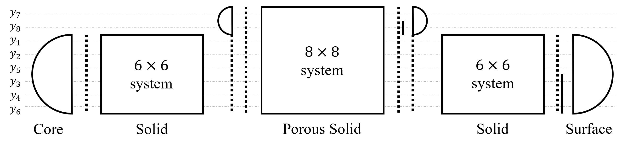
Note that for symmetry reasons I have reordered the $y$-functions. This way when we embed the $6\times6$ system in the $8\times8$ system we split the lower and upper parts and add one new porous $y$-function to both sets. If we had not done this, then the new grouping would contain 4 old and 2 old + 2 new $y$-functions, instead of 3 old + 1 new and 3 old + 1 new. Within the code we create a transfer matrix array $R$ (length $N$) with size $8 \times 8$, we subsequently expose the $6\times 6$ system as a "view". The specific ording as seen by the two systems is

\[\begin{aligned} \pmb{y}_{n,m} &= (U_{n,m} , V_{n,m} , \Phi_{n,m} , X_{n,m} , Y_{n,m}, \Psi_{n,m})^T & (6\times6) \\ \pmb{y}_{n,m} &= (U_{n,m} , V_{n,m} , \Phi_{n,m} , P_{n,m}, X_{n,m} , Y_{n,m}, \Psi_{n,m}, R_{n,m})^T & (8\times8) \end{aligned}\]

With this clarified, let us have a look at the diagram.

From the left, we start with the core solution boundary

\[ B = \begin{pmatrix} 1 & 0 & 0 & b_{11} & b_{12} & b_{13} \\ 0 & 1 & 0 & b_{21} & b_{22} & b_{23} \\ 0 & 0 & 1 & b_{31} & b_{32} & b_{33} \end{pmatrix},\]

We than impose continuity between $B$ and our modal solution vector, this is denoted by the dotted vertical line.

\[\begin{pmatrix} 1 & & & & & \\ & 1 & & & \\ & & 1 & & \\ & & & 1 & \\ & & & & 1 \\ & & & & & 1 \end{pmatrix}_{(6\times6)} \pmb{y}_{n,m}(r_1^-) = \begin{pmatrix} 1 & & & & & \\ & 1 & & & \\ & & 1 & & \\ & & & 1 & \\ & & & & 1 \\ & & & & & 1 \end{pmatrix}_{(6\times6)} \pmb{y}_{n,m}(r_C^+)\]

We then start constructing $R_n$ throughout the solid layers

\[ \pmb{C}_n \pmb{y}_n + \pmb{D}_{n+1} \pmb{y}_{n+1} = \pmb{0}\]

with $\pmb{A}_n$ the $6 \times 6$ motion matrix. At some point we encounter a porous layer, at this point we introduce the porous $y$-functions. We will introduce them in a decoupled fashion and allow them to couple to the $6 \times 6$ system in a minute. First we need to introduce an infinitesimal layer over which we impose continuity

\[\begin{pmatrix} 1 & & & & & & & \\ & 1 & & & & & & \\ & & 1 & & & & & \\ & & & 1 & & & & \\ & & & & 1 & & & \\ & & & & & 1 & & \\ & & & & & & 1 & \\ & & & & & & & 1 \end{pmatrix}_{(8\times8)} \pmb{y}_{n,m}(r_i^+) + b(r_i^+) = \begin{pmatrix} 1 & & & & & \\ & 1 & & & \\ & & 1 & & \\ & & & & & \\ & & & 1 & \\ & & & & 1 \\ & & & & & 1 \\ & & & & & \end{pmatrix}_{(8\times6)} \pmb{y}_{n,m}(r_i^-)\]

Evidently, for the LHS to have a zero on the 4th and 8th rows we must have

\[\begin{aligned} b_4(r_i^+) &= - y_4(r_i^+) \\ b_8(r_i^+) &= - y_8(r_i^+) \end{aligned}\]

while continuity of the $6 \times 6$ system implies that the other components of $b(r_i^+)$ are all zero. One may be inclined to put $b_4(r_i^+) = -1$ and $b_8(r_i^+) = 0$, i.e. none-zero pore pressure and zero Darcy flux, but there is a catch! These conditions only hold for the elementary solution, and not for the modal solution. Instead we would have to put $b_7(r_i^+) =-a_4$ and $b_8(r_i^+) = 0$, but what is $a_4$? Since we eliminated all weights already at the core this boundary is not very useful. Actually, let us try the following

\[\begin{aligned} b_4(r_i^+) &= -y_4(r_i^+) \\ b_8(r_i^+) &= 0 \end{aligned}\]

and treat $y_4(r_i^+)$ as some undetermined quantity.

This will enter into the equations as follows

\[\begin{pmatrix} B_1 \\ C_1 & D_2 \\ & C_2 & D_3 \\ &&\ddots & \ddots \\ &&&C_{i-1} & D_i \\ &&&&C_{i}^- & D_i^+ \\ &&&&& C_{i} & D_{i+1} \\ &&&&&&\ddots & \ddots \\ &&&&&&& C_{N-1} & D_N \\ &&&&&&&&B_N \end{pmatrix} \begin{pmatrix} \pmb{y} (r_C^+) \\ \pmb{y} (r_2) \\ \pmb{y} (r_3) \\ \vdots \\ \pmb{y} (r_i^-) \\ \pmb{y} (r_i^+) \\ \pmb{y} (r_{i+1}) \\ \vdots \\ \pmb{y}(r_{N-1}) \\ \pmb{y}(r_N) \end{pmatrix} = \begin{pmatrix} 0 \\ 0 \\ 0 \\ \vdots \\ 0 \\ b(r_i^+) \\ 0 \\ \vdots \\ 0 \\ b \end{pmatrix},\]

where

\[C_{i}^- = \begin{pmatrix} 1 & & & & & \\ & 1 & & & \\ & & 1 & & \\ & & & & & \\ & & & 1 & \\ & & & & 1 \\ & & & & & 1 \\ & & & & & \end{pmatrix}_{(8\times6)} \qquad \text{and} \qquad D_i^+ = -\begin{pmatrix} 1 & & & & & & & \\ & 1 & & & & & & \\ & & 1 & & & & & \\ & & & 1 & & & & \\ & & & & 1 & & & \\ & & & & & 1 & & \\ & & & & & & 1 & \\ & & & & & & & 1 \end{pmatrix}_{(8\times8)}\]

At this point we need to make sure also include the inhomogeneous part ($b_4(r_i^+)$ and $b_8(r_i^+)$) in our forwarding scheme. The governing equations change slightly, and we need to be careful about the dimensions of the matrices involved in the calculation around the interface. In order to not accidentally remove information from the systems, we shall embed the $6\times6$ system in the $8\times8$ space. For some matrix $M$ this implies

\[M_{(3\times6)} = \begin{bmatrix} a_1 & b_1 & c_1 & d_1 & e_1 & f_1 \\ a_2 & b_2 & c_2 & d_2 & e_2 & f_2 \\ a_3 & b_3 & c_3 & d_3 & e_3 & f_3 \\ \end{bmatrix}_{(3\times6)} \Rightarrow M_{(4\times8)} = \begin{bmatrix} a_1 & b_1 & c_1 & 0 & d_1 & e_1 & f_1 & 0 \\ a_2 & b_2 & c_2 & 0 & d_2 & e_2 & f_2 & 0 \\ a_3 & b_3 & c_3 & 0 & d_3 & e_3 & f_3 & 0 \\ 0 & 0 & 0 & 0 & 0 & 0 & 0 & 0 \\ \end{bmatrix}_{(4\times8)}\]

Applying this logic to $C^{l}_{i-1}$ and ${C_i^-}^{u}$

\[P_i^- \equiv \begin{bmatrix} C^{l}_{i-1} \\ 0 \end{bmatrix}_{(8\times8)}\]

\[S_i^- \equiv \begin{bmatrix} D^{l}_i \\ {C_i^-}^{u} \end{bmatrix}_{(8\times8)}\]

\[Q_i^- \equiv \begin{bmatrix} 0 \\ {D_i^+}^{u} \end{bmatrix}_{(8\times8)}\]

We now obtain an $R_i^-$ matrix with dimensions $8 \times 8$. Now we need to figure out how the $8 \times 8$ system departs from the interface. Lets start by considering the governing equation for a system with internal boundary

\[\left(P_n R_{n-1} + S_n \right) y_n + Q_n y_{n+1} = b_n.\]

We can reformulate this specifically for the interface layer as

\[\left(P_i^+ R_{i}^- + S_i^+ \right) y_i^+ + Q_i^+ y_{i+1} = b(r_i^+)\]

where

\[P_i^+ \equiv \begin{bmatrix} {C_{i}^-}^{l} \\ 0 \end{bmatrix}\]

Again, we need to be careful here given the odd dimensions of ${C_{i}^-}^{l}$. The continuity of the porous $y$-functions into their own $2\times2$ system implies that we expand ${C_{i}^-}$ into the $8 \times 8$ identity matrix (as seen from the porous layer). We thus have $P_i^+$ with dimensions $8 \times 8$. Next

\[S_i^+ \equiv \begin{bmatrix} {D_i^+}^{l} \\ {C_{i+1}}^{u} \end{bmatrix}\]

is trivial, and similarly

\[Q_i^+ \equiv \begin{bmatrix} 0 \\ {D_{i+1}}^{u} \end{bmatrix}\]

is trivial, both are $8 \times 8$ matrices.

We can now plug everything in and simplify

\[\begin{aligned} \left(P_i^+ R_{i}^- + S_i^+ \right) y_i^+ + Q_i^+ y_{i+1} &= b(r_i^+) \end{aligned}\]

Recall that $b(r_i^+)$ depends on $y_i^+$, we may write $b(r_i^+) = K y_i^+$ where $K$ extracts the 7th and 8th components of $y_i^+$ and changes the sign. We thus write

\[\begin{aligned} \left(P_i^+ R_{i}^- + S_i^+ + K\right) y_i^+ &= - Q_i^+ y_{i+1} \\ y_i^+ &= - \left(P_i^+ R_{i}^- + S_i^+ + K\right)^{-1} Q_i^+ y_{i+1} \\ &= R_i^+ y_{i+1} \end{aligned}\]

With these conditions on $\pmb{1}$ and $K$ we can determine the interface form of the equations.

However, we should be careful not to accidentally store too much information in $R_i^-$ and $R_i^+$. Realize that we embedded the $6 \times 6$ system in an $8 \times 8$ space to construct a square and invertible matrix $X_i^-$. This came at the cost of padding the matrices with zeros. If one instead combined the non-square matrices, they would obtain $R_i^-$ with size $6 \times 8$

\[\begin{aligned} P_i^- \cdot R_{i-1} + S_i^- &= X_i^- \\ (7 \times 6) \cdot (6 \times 6) + (7 \times 6) &\Rightarrow (7 \times 6) \\ -(X_i^- )^{-1} Q_i^- &= R_i^- \\ (6 \times 7) \cdot (7 \times 8) &\Rightarrow (6 \times 8) \end{aligned}\]

Hence, at this step the rows corresponding to $y_7$ and $y_8$ to zero. Next we repeat these steps and include the internal boundary condition on $y_7$

\[\begin{aligned} P_i^+ \cdot R_i^- + S_i^+ + K &= X_i^+ \\ (8 \times 6) \cdot (6 \times 8) + (8 \times 8) + (8 \times 8) &\Rightarrow (8 \times 8) \\ -(X_i^+ )^{-1} Q_i^+ &= R_i^+ \\ (8 \times 8) \cdot (8 \times 8) &\Rightarrow (8 \times 8) \end{aligned}\]

The resulting system contains now information on $y_8$ from below, hence we must set the row corresponding to $y_8$ to zero in $R$. This closes the system and accounts for all dof.

Now we proceed constructing $R_n$ through the porous layers

\[ \pmb{C}_n \pmb{y}_n + \pmb{D}_{n+1} \pmb{y}_{n+1} = \pmb{0}\]

with $\pmb{A}_n$ the $8 \times 8$ motion matrix.

When we reach the top of the porous layers, potentially at the surface, but maybe sooner, we need to decouple $y_7$ and $y_8$ from the $6 \times 6$ system. Impose again an infinitesimal layer

\[\begin{pmatrix} 1 & & & & & \\ & 1 & & & \\ & & 1 & & \\ & & & & & \\ & & & 1 & \\ & & & & 1 \\ & & & & & 1 \\ & & & & & \end{pmatrix}_{(8\times6)} \pmb{y}_{n,m}(r_i^+) + b(r_i^+) = \begin{pmatrix} 1 & & & & & & & \\ & 1 & & & & & & \\ & & 1 & & & & & \\ & & & 1 & & & & \\ & & & & 1 & & & \\ & & & & & 1 & & \\ & & & & & & 1 & \\ & & & & & & & 1 \end{pmatrix}_{(8\times8)} \pmb{y}_{n,m}(r_i^-)\]

Here we apply the constraint that the Darcy flux vanishes at the interface. The pore pressure remains unconstrained. Evidently, for the RHS to have a zero on the 8th row we must have

\[\begin{aligned} b_7(r_i^+) &= y_7(r_i^-) \\ b_8(r_i^+) &= 0 \end{aligned}\]

Similar to before, this interface will enter into the equations as follows

\[\begin{pmatrix} B_1 \\ C_1 & D_2 \\ & C_2 & D_3 \\ &&\ddots & \ddots \\ &&&C_{i-1} & D_i \\ &&&&C_{i}^- & D_i^+ \\ &&&&& C_{i} & D_{i+1} \\ &&&&&&\ddots & \ddots \\ &&&&&&& C_{N-1} & D_N \\ &&&&&&&&B_N \end{pmatrix} \begin{pmatrix} \pmb{y} (r_C^+) \\ \pmb{y} (r_2) \\ \pmb{y} (r_3) \\ \vdots \\ \pmb{y} (r_i^-) \\ \pmb{y} (r_i^+) \\ \pmb{y} (r_{i+1}) \\ \vdots \\ \pmb{y}(r_{N-1}) \\ \pmb{y}(r_N) \end{pmatrix} = \begin{pmatrix} 0 \\ 0 \\ 0 \\ \vdots \\ 0 \\ b(r_i^+) \\ 0 \\ \vdots \\ 0 \\ b \end{pmatrix},\]

where

\[C_{i}^- = \begin{pmatrix} 1 & & & & & & & \\ & 1 & & & & & & \\ & & 1 & & & & & \\ & & & 1 & & & & \\ & & & & 1 & & & \\ & & & & & 1 & & \\ & & & & & & 1 & \\ & & & & & & & 1 \end{pmatrix}_{(8\times8)} \qquad \text{and} \qquad D_i^+ = -\begin{pmatrix} 1 & & & & & \\ & 1 & & & \\ & & 1 & & \\ & & & 1 & \\ & & & & 1 \\ & & & & & 1 \\ & & & & & \\ & & & & & \end{pmatrix}_{(8\times6)}\]

Again we will pad some of the matrices where necessary

\[P_i^- \equiv \begin{bmatrix} C^{l}_{i-1} \\ 0 \end{bmatrix}\]

\[S_i^- \equiv \begin{bmatrix} D^{l}_i \\ {C_i^-}^{u} \end{bmatrix}\]

\[Q_i^- \equiv \begin{bmatrix} 0 \\ {D_i^+}^{u} \end{bmatrix}\]

and apply the conditions on $\pmb{1}$ and $K$ to obtain the interface form of the equations. (This is still a partial work in progress, however it seems to work in the numerical implementation.) A simply work around these interfaces is to assign a porosity slightly greater than the porosity threshold in the code, this way the solver will be constructed as purely mush propagator without interfaces.

The model implementation has been tested and has been found internally consistent for forcing frequencies between $10^{-4}$ and $10^{-6}$ Hz. This range may be extended when the non-dimensionalization is properly implemented, or when the interface conditions are behaving as expected.